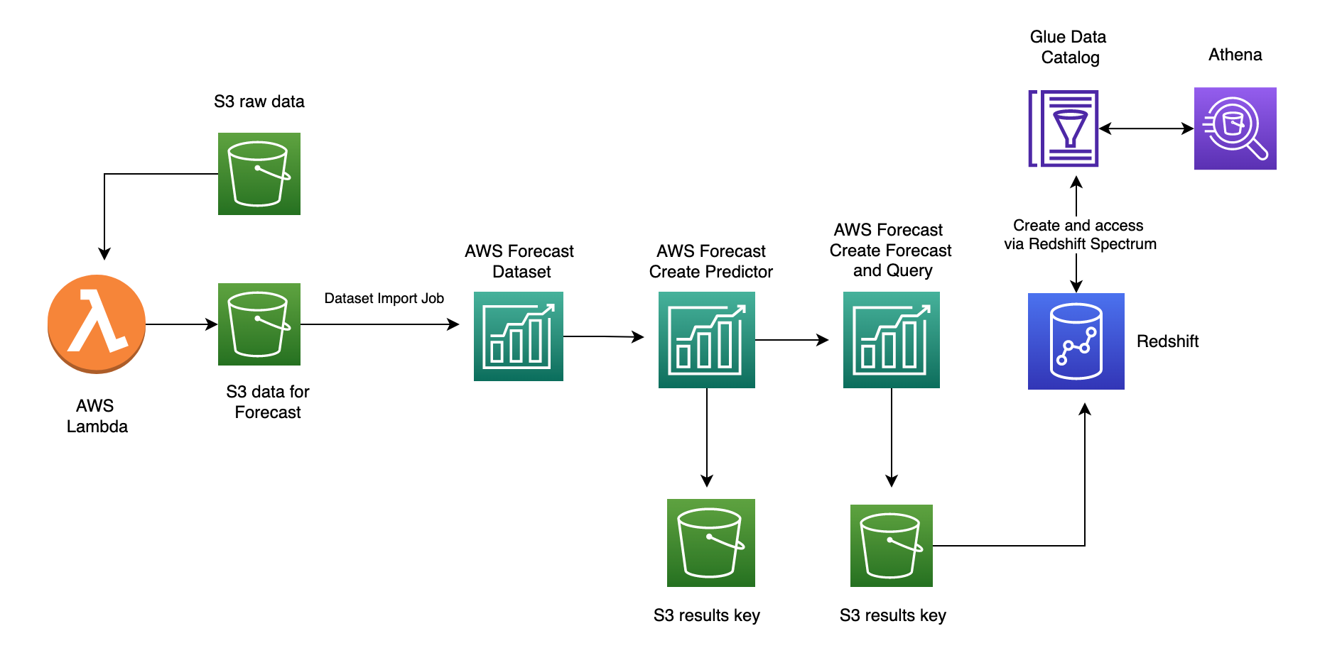
Forecasting American Football Fever in AWS using Wikipedia Page Hits

---

Forecast is a fully managed AWS service for time-series analysis. It can select from multiple time series prediction models to find the best one for your particular data sets. Amazon Forecast automatically examines the historical data provided (including any additional features that can impact the forecast), and identify what is meaningful, and produce a forecasting model capable of making highly accurate predictions.

Illustrating the use of AWS Forecasts service using the Manning Dataset. This is part of the FbProphet Library example dataset which is a time series of the Wikipedia search frequencies (log- transformed) for Peyton Manning taken over an 8 year period [8]. American Football begins in Septemeber and ends in early January every year, with playoffs scheduled thereafter. Games tend to be televised on Sunday and Monday nights. By using historical data of wikipedia page hits of a popular player like Peyton Manning, we could model weekly and yearly seasonality of wikipedia page hits and use that as an indication of football hype. We may expect to see a lot more activity during the playoff season and superbowl for example.

The modules and functions referenced in the code blocks in this exercise can be accessed here. These contain helper functions for importing data into S3, creating an AWS forecast dataset and importing data into it from S3, training a predictor and then forecasting using the model. The code snippets and outputs used in the next few sections, can also be accessed in the notebook. Instructions on configuring the virtual environment with dependencies can be accessed here.

Data preparation

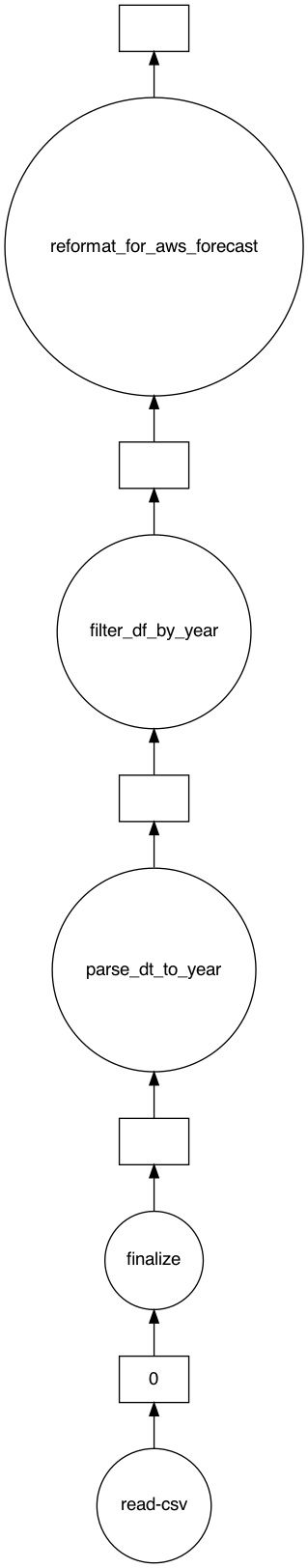
The functions in modules prepare_data_for_s3.py filter the existing dataset to only include historical data for one year (2015) and then reformat the dataset to have columns (“timestamp”, “target_value”,”item_id”) and values as expected by AWS Forecast api. Finally we call the s3 put object to add to created S3 bucket.

For illustration purposes and to generate the task viz, ive used dask delayed, but the dataset size certainly does not warrant the need for it.

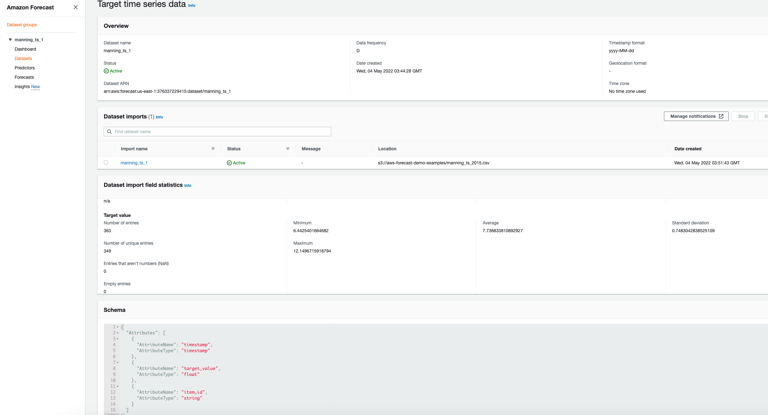
The filtered raw data for 2015 which is imported into S3 and then imported into AWS forecast has the following profile

Module dataset_and_import_jobs.py creates an AWS Forecast dataset group and dataset as described in AWS docs [1]. Here we only use target time series dataset type The dataset group must include a target time series dataset which includes the target attribute (item_id) and timestamp attribute, as well as any dimensions. Related time series and Item metadata is optional [1]

For the data uploaded to S3 using module prepare_data_for_s3.py, the itemid column has been created and set to arbitary value (1) as all the items belong to the same group (i.e Manning’s wikipedia hits)

The dataset group and import job can then be created using the snippet below after setting the data frequency for daily frequency and ts_schema. We can access all the forecast services apis via the boto client interface.

forecast = boto3.client("forecast")
DATASET_FREQUENCY = "D"
ts_schema ={
   "Attributes":[
      {
         "AttributeName":"timestamp",
         "AttributeType":"timestamp"
      },
      {
         "AttributeName":"target_value",
         "AttributeType":"float"
      },
      {
         "AttributeName":"item_id",
         "AttributeType":"string"
      }
   ]
}
PROJECT = 'manning_ts'
DATA_VERSION = 1

def create_dataset(dataset_name, freq, schema):
    response = forecast.create_dataset(
        Domain="CUSTOM",
        DatasetType="TARGET_TIME_SERIES",
        DatasetName=dataset_name,
        DataFrequency=freq,
        Schema=schema,
    )

    dataset_arn = response["DatasetArn"]
    print(forecast.describe_dataset(DatasetArn=dataset_arn))
    return dataset_arn
    
def create_dataset_group_with_dataset(dataset_name, dataset_arn):
    dataset_arns = [dataset_arn]
    try:
        create_dataset_group_response = forecast.create_dataset_group(
            Domain="CUSTOM", DatasetGroupName=dataset_name, DatasetArns=dataset_arns
        )
        dataset_group_arn = create_dataset_group_response["DatasetGroupArn"]
        return dataset_group_arn
    except forecast.exceptions.ResourceAlreadyExistsException:
        print("Dataset group already exists")


dataset_name = f"{PROJECT}_{DATA_VERSION}"
dataset_arn = create_dataset(dataset_name, DATASET_FREQUENCY, ts_schema)
dataset_group_arn = create_dataset_group_with_dataset(dataset_name, dataset_arn)

We then create an import job to import the time series dataset from s3 into AWS forecast dataset so it is ready for training. After creating the import job - we can check for job status before progressing to the training step

from dataset_and_import_jobs import create_import_job
from common import check_job_status

bucket_name = 'aws-forecast-demo-examples'
key = "manning_ts_2015.csv"

ts_dataset_import_job_response = create_import_job(bucket_name, key, dataset_arn, role_arn)
dataset_import_job_arn=ts_dataset_import_job_response['DatasetImportJobArn']
check_job_status(dataset_import_job_arn, job_type="import_data")

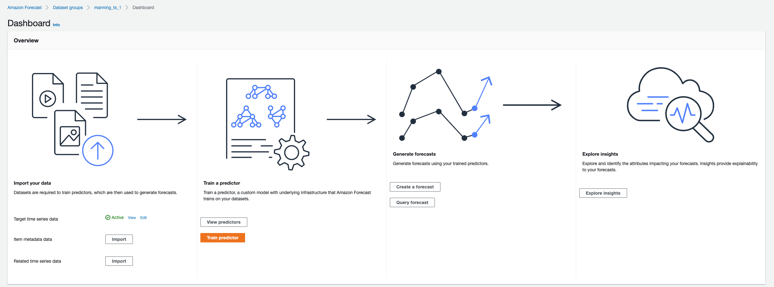
Model Training

Create a predictor (an Amazon Forecast model) that is trained using the target time series. You can use predictors to generate forecasts based on your time-series data.

Amazon Forecast requires the Dataset group, Forecast frequency and Forecast horizon inputs when training a predictor [2] Hence these are passed into the custom functions for creating the predictor, with the following settings:

• Dataset group (defined previously)
• Forecast frequency – The granularity of your forecasts (in this case daily).
• Forecast horizon – The number of time steps being forecasted (in this case, set this to 35 days)

This function runs automl by default, trains an optimal combination of algorithms to each time series in the dataset. However, if the auto_ml parameter is set to False, it will run manual selection based on the alogorithm parameter set. This defaults to ‘Non Parametric Time Series’ but can be overidden.
Note In the script, I am currently using the legacy predictor (CreatePredictor) api for manual selection. we can also upgrade to use AutoPredictor to create predictors as suggested in the AWS docs [2]. This has two advantages. Forecast Explainability and predictor retraining features are only available for predictors created with AutoPredictor. AutoPredictor is the default and preferred method to create a predictor with Amazon Forecast as the predictors are more accurate. It applies the optimal combination of algorithms to the time series in the dataset.[2]. If the script is run without changing any parameters, it will create predictors using AutoPredictor.

from create_predictor_forecast_jobs import train_aws_forecast_model
from common import check_job_status

FORECAST_LENGTH = 35
DATASET_FREQUENCY = "D"
predictor_name = f"{PROJECT}_{DATA_VERSION}_automl"

create_predictor_response , predictor_arn = train_aws_forecast_model(predictor_name, FORECAST_LENGTH, DATASET_FREQUENCY, dataset_group_arn)
check_job_status(predictor_arn, job_type="training")

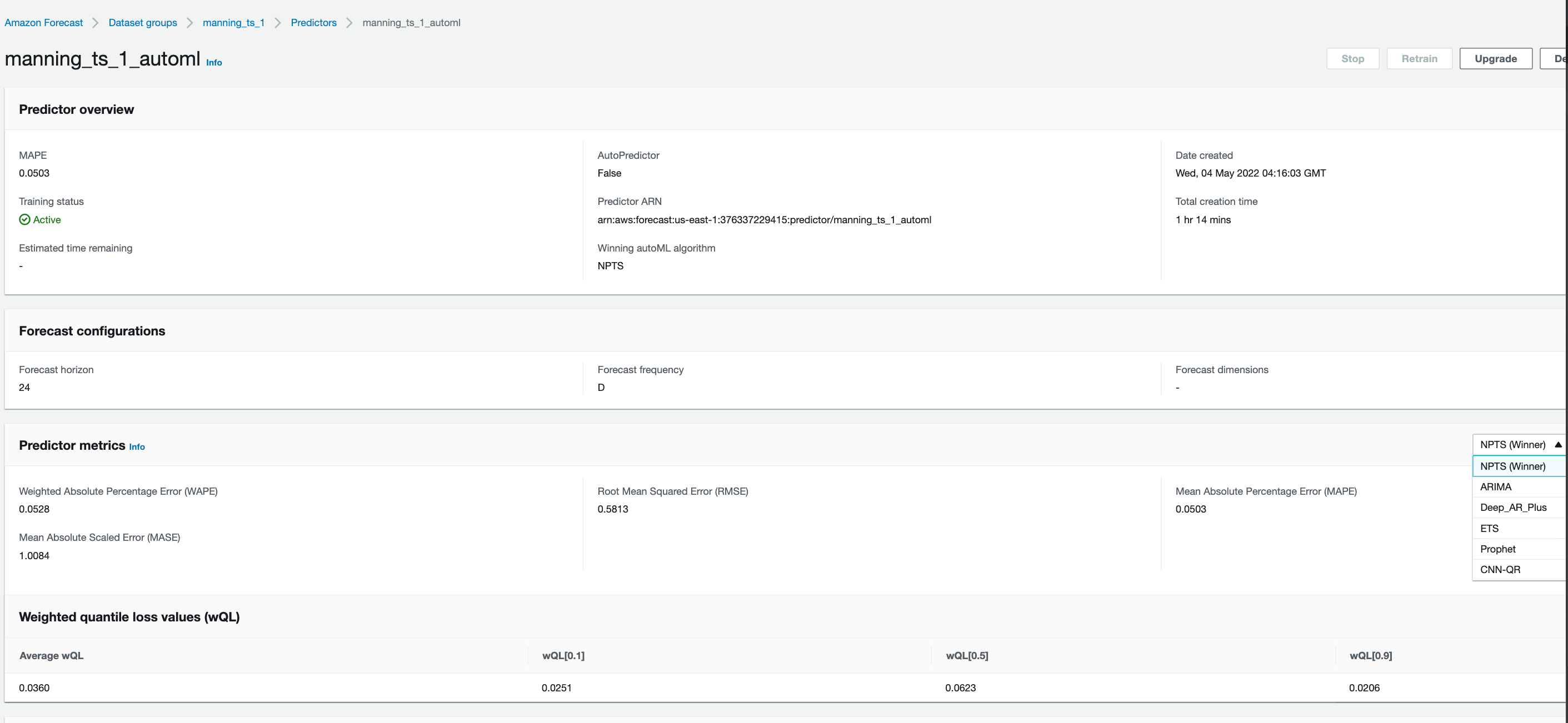
Backtest results

Amazon Forecast uses backtesting to compute metrics, for evaluating predictors. Some of these are listed below, along with the common use cases for applying each one [3].

Metric	Definition	When to use	equation
RMSE	square root of the average of squared errors. It is sensitive to large deviations (outliers) between the actual demand and forecasted values.	Useful in cases when you want to penalise outliers where a few large incorrect predictions from a model on some items can be very costly to the business. For sparse datasets where demand for items in historical data is low, it would be better to use WAPE or wQL instead as RMSE will not account for scale of total demand	$\frac{n}{T} \Sigma_{i,t}({y_{i,t}}-\hat{y_{i,t}})^2$
wQL	measures accuracy of a model at a specified quantile. An extension of this is the Average wQL metric which is the mean of wQL values for all quantiles (forecast types) selected during predictor creation.	wQL is particularly useful when there are different costs for underpredicting and overpredicting. By setting the weight of the wQL function, you can automatically incorporate differing penalties for underpredicting and overpredicting. The Average wQL can be used for evaluating forecasts at multiple quantiles together.	$2\frac{\Sigma_{i,t}[\tau\max(y_{i,t} - q_{i,t}^{(\tau)}, 0) + (1-\tau)\max(q_{i,t}^{(\tau)} - y_{i,t}, 0)]}{\Sigma_{i,t}\left| y_{i,t} \right|}$
MASE	divides the average error by a scaling factor which is dependent on the seasonality value, that is selected based on the forecast frequency. MASE is a scale-free metric, which makes it useful for comparing models from different datasets. MASE values can be used to meaningfully compare forecast error across different datasets regardless of the scale of total demand.	ideal for datasets that are cyclical in nature or have seasonal properties. e.g. forecasting for products that are in high demand in summer compared to winter	$\frac{\frac{1}{J} \Sigma_{j}( \left| {e_{j}} \right|)}{\frac{1}{T-m} \Sigma_{t=m+1}^{T}( \left| {Y_{t} - {Y_{t-m}}} \right|)} $
MAPE	percentage difference of the mean forecasted and actual value) averaged over all time points. The normalization in the MAPE allows this metric to be compared across datasets with different scales.	useful for datasets where forecasting errors need to be emphasised equally on all items regardless of demand. It also equally penalizes for under-forecasting or over-forecasting, so useful metric to use when the difference in costs of under-forecasting or over-forecasting is negligible	$\frac{1}{n} \Sigma_{i,t} \left| \frac{A_{t} - F_{t}}{A_{t}} \right| $
WAPE	sum of the absolute error normalized by the total demand. A high total demand results in a low WAPE and vice versa.The weighting allows these metrics to be compared across datasets with different scales.	useful in evaluating datasets that contain a mix of items with large and small demand. A retailer may want to prioritise forecasting errrors for standard items with high sales compared to special edition items which are sold infrequently. WAPE would be a good choice in such a case. For sparse datasets where a large proportion of products are sold infrequently (i.e. demand is 0 for most of the historical data), WAPE would be a better choice compared to RMSE as it accounts for the total scale of demand.	$\frac{ \Sigma_{i,t}({y_{i,t}}-\hat{y_{i,t}})^2}{\Sigma_{i,t}({y_{i,t}}})$

The metrics are provided for each backtest window specified. For multiple backtest windows, the metrics are averaged across all the windows. The user can adjust the backtest window length (testing set) and the number of backtests (can vary from 1 to 5) when training a predictor [3]. However, the backtest window length must be at least as large as the prediction window or forecast horizon (this is the default setting if not overriden by the user). It also cannot exceed more that half the length of the entire time series. The metrics are computed from the forecasted values and observed values during backtesting. Missing values which are filled in the dataset using one of the AWS forecast supported methods [4], are not used when computing the metrics as they are not classed as observed values [3].

We can generate the backtesting metrics by calling the function with the predictor_arn value, which calls the get_accuracy_metrics method from the forecast api.

from create_predictor_forecast_jobs import evaluate_backtesting_metrics
error_metrics = evaluate_backtesting_metrics(predictor_arn)

We can also plot the backtest results for all the metrics.

import numpy as np
import json

def plot_backtest_metrics(error_metrics):
    parsed_json = {
        "Algorithm": [],
        "WQuantLosses": [],
        "WAPE": [],
        "RMSE": [],
        "MASE": [],
        "MAPE": [],
        "AvgWQuantLoss": [],
    }
    for v in error_metrics:
        algo = v["AlgorithmArn"].split("/")[-1]
        weighted_quantile_losses = v["TestWindows"][0]["Metrics"][
            "WeightedQuantileLosses"
        ]
        wape = v["TestWindows"][0]["Metrics"]["ErrorMetrics"][0]["WAPE"]
        rmse = v["TestWindows"][0]["Metrics"]["ErrorMetrics"][0]["RMSE"]
        mase = v["TestWindows"][0]["Metrics"]["ErrorMetrics"][0]["MASE"]
        mape = v["TestWindows"][0]["Metrics"]["ErrorMetrics"][0]["MAPE"]
        avg_weighted_quantile_losses = v["TestWindows"][0]["Metrics"][
            "AverageWeightedQuantileLoss"
        ]
        parsed_json["Algorithm"].append(algo)
        parsed_json["WQuantLosses"].append(json.dumps(weighted_quantile_losses))
        parsed_json["WAPE"].append(np.round(wape, 4))
        parsed_json["RMSE"].append(np.round(rmse, 4))
        parsed_json["MASE"].append(np.round(mase, 4))
        parsed_json["MAPE"].append(np.round(mape, 4))
        parsed_json["AvgWQuantLoss"].append(np.round(avg_weighted_quantile_losses, 4))
    df = (
        pd.DataFrame(parsed_json)
        .set_index("Algorithm")
        .T.rename_axis("Metric", axis=0)
        .rename_axis(None, axis=1)
        .reset_index()
    )
    df.iloc[1::, :].plot(x="Metric", kind="bar", figsize=(15, 8), legend=True)
    return df

plot_backtest_metrics(error_metrics)

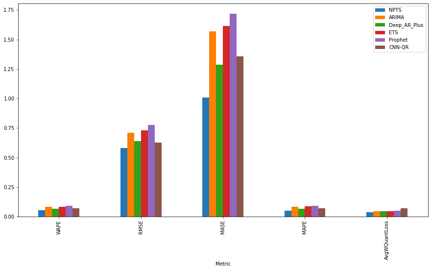
Looking at the results, seems like NPTS is the winning algorithm followed by Deep AR Plus. So AWS Forecast, will use the NPTS model for serving forecasts. We can also see MASE metric better highlights the difference in performance between various algorithms as it is more suited to this dataset due to cyclical/seasonal properties in data

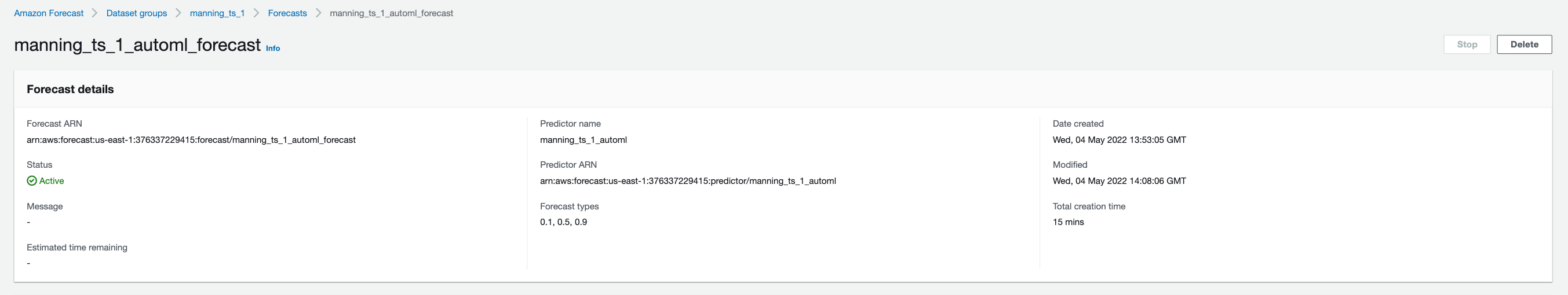
Forecast and query

Now we have a trained model so we can create a forecast. This includes predictions for every item (item_id) in the dataset group that was used to train the predictor [5]

from create_predictor_forecast_jobs import create_forecast

forecast_name = f"{PROJECT}_{DATA_VERSION}_automl_forecast"
forecast_arn = create_forecast(forecast_name, predictor_arn)

Once this is done, we can then query the forecast by passing a filter (key-value pair), where the key/values are one of the schema attribute names and valid values respectively. This will return forecast for only those items that satisfy the criteria [5]. In this case, we query the forecast and return all the items by using the item id dimension. We will use the forecast_arn value returned from the previous code block.

forecast = boto3.client("forecast")
forecastquery = boto3.client(service_name="forecastquery")

def run_forecast_query(forecast_arn, filters):
    forecast_response = forecastquery.query_forecast(
        ForecastArn=forecast_arn, Filters=filters
    )
    return forecast_response["Forecast"]["Predictions"]

def create_forecast_plot(forecast_response):
    ts = {}

    timestamp = [k["Timestamp"] for k in forecast_response["p10"]]
    p10 = [k["Value"] for k in forecast_response["p10"]]
    p50 = [k["Value"] for k in forecast_response["p50"]]
    p90 = [k["Value"] for k in forecast_response["p90"]]

    ts["timestamp"] = timestamp
    ts["p10"] = p10
    ts["p50"] = p50
    ts["p90"] = p90
    df = pd.DataFrame(ts)
    df.plot(x="timestamp", figsize=(15, 8))
    return df
    
filters = {"item_id":"1"}
forecast_response = run_forecast_query(forecast_arn, filters)
create_forecast_plot(forecast_response)

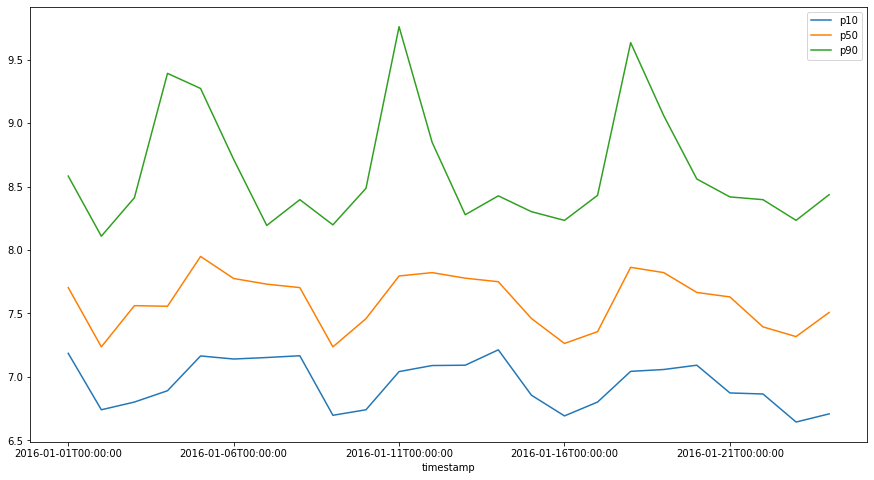
We can also further analyse the results stored in S3 directly from Athena or create external tables in Redshift Spectrum which reference database in Glue Data Catalog [6][7]. This will allow simple queries to be run without having to load data into Redshift tables. We can also query the data using Athena as it can access the Glue Data Catalog. When mapping data stored in S3 bucket as external tables, the path to the S3 file needs to be passed to the LOCATION parameter in the query.

Terminating resources

Finally we can tear down all the AWS Forecast resources: predictor, forecast and dataset group

from teardown_resource import delete_training_forecast_resources
kwargs = {'forecast':forecast_name,
'predictor':predictor_name
}

delete_training_forecast_resources(**kwargs)

References

1. Importing datasets https://docs.aws.amazon.com/forecast/latest/dg/howitworks-datasets-groups.html
2. Training Predictors https://docs.aws.amazon.com/forecast/latest/dg/howitworks-predictor.html
3. Predictor metrics and backtesting https://docs.aws.amazon.com/forecast/latest/dg/metrics.html
4. Handling missing values https://docs.aws.amazon.com/forecast/latest/dg/howitworks-missing-values.html
5. Generating and Querying forecasts https://docs.aws.amazon.com/forecast/latest/dg/howitworks-forecast.html
6. Query S3 data from Athena https://aws.amazon.com/blogs/big-data/analyzing-data-in-s3-using-amazon-athena/
7. Create External Tables Redshift Spectrum https://aws.amazon.com/premiumsupport/knowledge-center/redshift-spectrum-external-table/
8. Facebook Prophet paper using Manning dataset https://peerj.com/preprints/3190/