
Employee turnover is not only a cumbersome process but also a financial burden. Employers can benefit from knowledge of an employee’s likelihood of changing the company. Often, decisions for leaving a company do not emerge out of a sudden but are usually the outcome of careful pre-planning. Utilising a data-driven approach to analyse which employees are likely to leave the company soon, therefore, can be of great interest to managers. With the gained knowledge, human resource management teams can act upon these predictions to persuade employees to stay before they jump ship.
The following is analysis on carried out a Kaggle dataset using the Machine Learning Toolbox in Matlab, with the aim of predicting whether a employee is likely to leave the company or not. The dataset consists of 10 variables being a mixture of numerical and categorical variables. Table 1 depicts the individual features, their mean and standard deviation as well as categorical features and a target variable “Left” which consists of the two classes stay and leave. Furthermore, this dataset has ≈ 15.000 samples with a class imbalance of 11428 (stayed) and 3571 samples corresponding to “left”.
| Variable | Scaling | Mean | Standard Dev |
|---|---|---|---|
| Satisfaction level | Numerical | 0.61 | 0.25 |
| Last evaluation | Numerical | 0.76 | 0.17 |
| Number of Projects | Numerical | 3.8 | 1.23 |
| Avg. Monthly Hours | Numerical | 201 | 50 |
| Time Spend Company | Numerical | 3.5 | 1.46 |
| Work Accident | Numerical | 0.14 | 0.35 |
| Promotion last 5 years | Numerical | 0.02 | 0.144 |
| Sales (10 levels) | Categorical | N/A | N/A |
| Salary (low, med, high) | Categorical | N/A | N/A |
| Left (target variable) | Categorical | N/A | N/A |
As a next step, the dataset was explored by visualising a correlation heat map to gain a first intuition of predictive capability of our features. The correlation heat map displays the correlation between features themselves and the target variable.
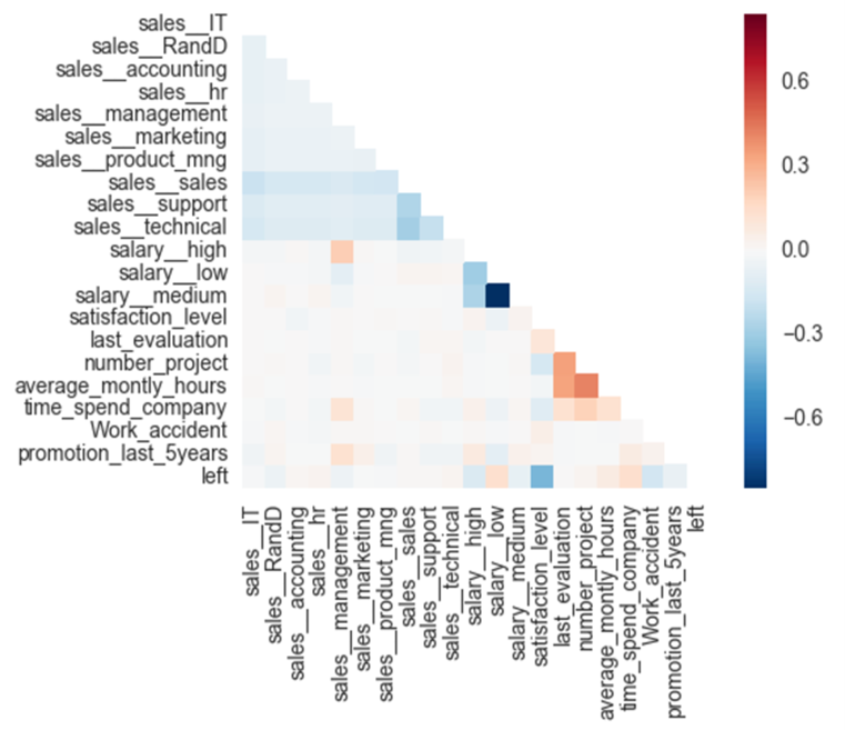
Most of the features show only very little correlation with each other as well as with our “left” target variable. One strong correlation can be observed between the target variable and the satisfaction level of approximately -0.5.
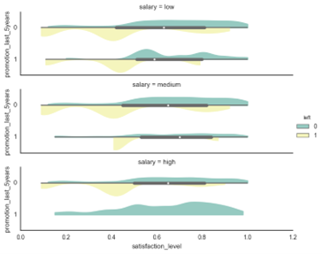
The violin plot shows the satisfaction level grouped by the salary and promotion_last_5years features. The yellow colour represents the employees which left the company. From this plot, we can conclude that the salary level is not a strong predictor but that some features such as salary and promotion_last_5years together can enhance our model’s predictive capability.
Some of the features, such as the Avg. hours per month lies on a much higher scale than the rest of the features. Therefore, the features were standardised to μ = 0 and σ = 1 to make sure that no feature is skewing the algorithm results towards the features on higher scales. We defined a scaling function in Matlab to output the scaled training data matrix as well as the corresponding μ and σ of every feature column.
1
2
3
4
5
6
7
8
9
10
11
12
13
14
15

function [Xscaled, mu, stddev] = scaler(X)
% This function standardizes the features to mu=0 and stddev=1.

Xscaled = X;
mu = zeros(1, size(X, 2));
stddev = zeros(1, size(X, 2));

% Perform feature scaling for every feature
for i=1:size(mu,2)
    mu(1,i) = mean(X(:,i)); % calculate the mean
    stddev(1,i) = std(X(:,i)); % calculate the stddev
    Xscaled(:,i) = (X(:,i)-mu(1,i))/stddev(1,i); % subtract the mean and devide by stddev
end
We call the function using the training data matrix and then use the μ and σ of the training data to standardise the test set.
1
2
3
4
5
6
7

[Xtrain, mu, stddev] = scaler(Xtrain);

for i=1:size(Xtest, 2)
    Xtest(:,i) = (Xtest(:,i)-mu(1,i))/stddev(1,i);
end
The two categorical features “salary” and “sales” had to be one-hot encoded and concatenated onto the numerical feature matrix. As a result, the feature matrix consists of shape 14999x21.
Algorithms
The choice of a given model depends on the dataset in question. Here we will explore Support Vector Machines (SVM) and MultiLayer Perceptron (MLP).
SVM is a supervised algorithm used for classification and regression tasks. A decision boundary is computed which maximises the distance from the data points closest to the decision boundary, also known as support vectors [12]. Given a training set, the optimal decision boundary is computed which separates the classes with a geometric margin or ‘gap’ such that it results in good and confident predictions on the samples [12]. MLP is a supervised feedforward learning algorithm that learns functions in an unsupervised fashion through its hidden layers and activation functions to map the input in the training data to an output [6] [13]. The hidden layer transforms the values from the inputs neurons in the leftmost layer with a weighted linear summation followed by an activation function which maps the values [9]. These values are received by the output layer which transforms them into output values by utilising a linear combination (regression) or a sigmoid function (binary classification) [6]. Through backpropagation, we gain the partial derivatives of our loss function w.r.t. the weights and use these to adjusts the weights through gradient descent. This process is repeated over a specified number of epochs and until we reach a certain minimum of the loss function [6].
There are several advantages and disadvantages of using each of the models, which have been summarised below:
| SVM | MLP | |
|---|---|---|
| Pros | 1. Effective for high dimensional problems | 1. Unsupervised feature learning through hidden layers and non-linear activation functions |
| 2. Memory efficient: uses a few training points (support vectors) for computing the decision boundary | 2. Powerful algorithm for numerous different kinds of data sets, especially perceptual data | |
| Cons | 1. Does not perform well if there is too much noise in the dataset | 1. Requires large amounts of data and computational resources |
| 2. Depending on the chosen kernel, training and testing time can be very slow | 2. Computationally expensive as a number of hyperparameters need to be tuned |
Training and evaluation methodology
Modelling was carried out in MATLAB (version 2016b) using the functions in the Neural Network Toolbox [9] for MLP implementation and Statistics and Machine Learning Toolbox [10] for SVM implementation. As a first step, we split our data into 70% training and 30% test set which is important to evaluate the generalisation performance in an unbiased way.
1
2
3
4
5
6
7
8
9
10
11
12
13

% load data and shuffle
df = importdata('data_clean.csv');
rng(10);
n = randperm(length(df));
data = df(n, :);  % permuatation

% Split data set into 70 % training and 30 % testing
Xtrain = data(1:10500, 1:20);
Xtest = data(10501: end, 1:20);
ytrain = data(1:10500, end);
ytest = data(10501:end, end);
After this, for both SVM and MLP, we applied grid search for hyper parameter tuning embedded in a 5-fold stratified cross validation. Throughout the grid search procedure, we used misclassification rate as a performance metric provided by the grid search hyper parameter tuning function. After grid search, the models with the optimal HP were retrained on the full training data. For the test set evaluation, we relied on a confusion matrix, and especially the recall score, which is helpful in our case of identifying how many samples our models can correctly classify as left out of all samples that correspond to “left” (the true positive rate).
Grid Search
Following the data pre-processing steps discussed in the previous section, both SVM and MLP were tuned with their distinct HP values. For SVM, the tuning process was split into distinct steps to reduce the amount of computing needed for HP tuning: First, grid search was applied over different kernel functions (linear, Gaussian, polynomial). Subsequently, randomised grid search was utilised to tune the specific kernel parameters C (Box Constraint) and σ (Kernel Scale) over a range of possible parameter values.
- Kernel function (first round): [linear, Gaussian, polynomial]
- Box Constraint (second round): [0.1 – 1]
- Kernel Scale (second round): [0.1 – 1]
We chose to utilise randomised search [1] to speed up the the enormous compute time needed to tune these parameters. Also, from initial experiments, we could observe that close values around the default parameters of C and σ worked best. For both C and σ, we chose therefore to tune between a range of 0.1 and 1 with a step size of 0.1.
1
2
3
4
5
6
7
8
9
10
11
12
13
14
15
16
17
18
19
20
21
22
23
24
25
26
27
28
29
30
31
32
33
34
35
36
37
38
%1) HP grid search 1) Search for best kernel function between linear,
%gaussian and polynomial kernels

% Create random partition for stratified 5-fold cross validation. Each fold
% roughly has the same class proportions.

cv = cvpartition(ytrain,'Kfold',5);

% loop over different kernel functions with 5 fold stratified cross
% validation
for i = {'linear', 'gaussian', 'polynomial'}
    % fitcecoc requires an SVM template
    t = templateSVM('KernelFunction', i{1});
    svm = fitcecoc(Xtrain, ytrain, 'learners', t, 'CVPartition', cv);
    accuracy = 1- kfoldLoss(svm);
    fprintf('\nAccuracy score of SVM with %s Kernel: %0.2f %', i{1}, accuracy)
end

% results:
%Accuracy score of SVM with linear Kernel: 0.78
%Accuracy score of SVM with gaussian Kernel: 0.97
%Accuracy score of SVM with polynomial Kernel: 0.95

%% Continue with gaussian kernel and tune C and sigma

% create HP object
params = hyperparameters('fitcecoc', Xtrain, ytrain, 'svm');
% change range of C
params(2).Range = [0.1, 1];
% change range of sigma
params(3).Range = [0.1, 1];

% fit random search
fitcecoc(Xtrain, ytrain, 'OptimizeHyperparameters', params,...
    'HyperparameterOptimizationOptions',struct('AcquisitionFunctionName',...
    'expected-improvement-plus', 'Optimizer', 'randomsearch', 'MaxObjectiveEvaluations',...
    10, 'CVPartition', cv));
Such as with SVM, a HP grid search was conducted with MLP as well. The Neural Computing Toolbox [9]does not implement a grid search so this had to be coded in manually. The first two parameters set the number of hidden neurons in each layer and the number of layers. The higher this value, the more capacity the network has to model complex input distributions [6]. A range of values have been chosen for the learning rate. The smaller the learning rate, the longer it takes to reach the minimum of the error function [6]. Conversely, if the learning rate is too large, there is a possibility of the weight updates diverging from the error minimum.
The chosen HP tuning range for MLP are listed below
- Number of hidden neurons: [60, 100]
- Number of layers: [3, 7]
- Learning rate: [0.01, 0.1, 0.9]
During the HP tuning of the MLP, a fast algorithm based on Scaled Conjugate Gradient (SCG) backpropagation method [11], developed by Moller, for updating weights and bias values was chosen. The traditional backpropagation algorithms, adjust the weights in the direction the gradient is decreasing the fastest. This does not necessarily result in fastest convergence. By searching along the conjugate direction compared to the steepest gradient direction, quicker convergence is achieved [11]. The error in classification is minimised using the mean square error.
Furthermore, early stopping is also implemented to stop training before the maximum number of epochs is reached [2]. This prevents the algorithm from overfitting on the training data and improves generalisation [2]. In this case, the algorithm stops if the validation error does not decrease for 6 consecutive epochs.
The Matlab code for implementing this is below:
1
2
3
4
5
6
7
8
9
10
11
12
13
14
15
16
17
18
19
20
21
22
23
24
25
26
27
28
29
30
31
32
33
for hiddenLayerSize = [10 20 40 60 80];  % number of hidden neurons
epochs = 500; % maximum number of epochs
for lr = [0.05 0.1 0.3 0.6 0.9]; % learning rate
for numLayers = [3 5 7];  % number of layers in the MLP
net = feedforwardnet(hiddenLayerSize, 'trainscg'); % Stochastic conjugate gradient
net.trainParam.epochs = epochs;	% Maximum number of epochs to train
net.trainParam.lr = lr; % learning rate
net.trainParam.goal = 0.01;	% stop training if error gold reached
net.numLayers = numLayers; % number of layers in the MLP
% generate cross validation indices for partition of data into 5 folds
indices = crossvalind('Kfold',x_train(1,:),5);
performance_cv = zeros(1,5);
for j = 1:5  % for each fold
    % samples which are present in fold j are true
      testIdx = (indices == j); % boolean vector of test indices
      trainIdx = ~testIdx  ; % boolean vector of train indices (which are not test)
      trInd = find(trainIdx); % get training sample indices
      tstInd = find(testIdx); % get test sample indices

net.divideFcn = 'divideind'; % dividing the samples into sets using indices
net.divideParam.trainInd=trInd; % separate samples into train set using train indices
net.divideParam.testInd=tstInd; % separate samples into test set using test indices

% Train the Network
[net,tr] = train(net, x_train, t_train);

% Fit the model on the training data
pred_cv = net(x_train);
% calculate the difference between predicted and target values
e = gsubtract(t_train, pred_cv);
% compute performance of the network for a single fold
performance_cv(:,j) = perform(net,t_train,pred_cv);
Hyper parameter optimisation results
Both SVM and MLP were tuned on the defined grids described in the previous section. For SVM, the best performing kernel was the Gaussian kernel (with default values for C and σ of 1) and resulted in a very high training accuracy score of 98.9%. The linear kernel (accuracy of 78%) was far behind the Gaussian and polynomial kernel (95% accuracy). Therefore, we continued to tune the SVM with Gaussian kernel further in its box constraint (C) parameter and kernel size (σ) with a random search using 5-fold cross validation and 10 random picks. From Table 4 we can observe, that randomised grid search resulted in a σ of 0.16 and a C parameter value of 0.28. This setting, however, led to a strong decrease in accuracy score of 86%. As such, the default values of 1, for σ and C (which resulted in a training accuracy score of 97%) were chosen as the parameters for retraining SVM on the full training set leading to an accuracy score of 98.8%.
1
2
3
4
5
6
7
% train on best HP values
t = templateSVM('KernelFunction', 'gaussian', 'KernelScale', 1, 'BoxConstraint', 1);
rng(10);
svm = fitcecoc(Xtrain, ytrain, 'learners', t);
% compute loss
train_error_svm = loss(svm, Xtrain, ytrain);
fprintf('\nSVM train accuracy: %0.2f\n', (1 - train_error_svm) * 100)
For the MLP, the optimal parameters were found to be: Number of neurons 60, number of layers: 3 and learning rate: 0.1. MLP was retrained with a more robust backpropagation method invented by MacKay in 1992 [8] which is computationally more expensive but more accurate than the SCG method [5]. This network function performs Bayesian Regularisation (BR) [5] [8] by implementing the Levenberg-Marquardt algorithm [5], to minimise the weights and biases so that the model generalises well.
1
2
3
4
5
6
7
8
9
10
11
12
13
14
15
16
17
18
19
20
21
22
23
24
25
26
27
28
29
30
31
32
33

% total time for training model with best HP: ~30 mins

trainFcn = 'trainbr' % Here we apply a more robust method: Bayesian Regularisation Backpropagation
hiddenLayerSize =60;  % number of hidden neurons
epochs = 500; % maximum number of epochs
lr = 0.1; % learning rate
numLayers = 3;
% creating a MLP object setting hidden layer size and backprop algorithm
net = feedforwardnet(hiddenLayerSize, trainFcn);

% setting other parameters for the MLP

net.trainParam.epochs = epochs;	% Maximum number of epochs to train
net.trainParam.lr = lr; % learning rate
net.trainParam.goal = 0.01;	% stop training if error gold reached
net.numLayers  = numLayers; % number of layers in MLP
% Setup Division of Data for Training, Validation, Testing
net.divideParam.trainRatio = 70/100; % keep 70% of data for training the model
net.divideParam.valRatio = 30/100; % keep 30% of the training data for model evaluation

% Evaluate the Network on the tr
[net,tr] = train(net, x_train, t_train);

% fit the model to the training data
pred_train = net(x_train);
% compute the difference between the train and predicted
e = gsubtract(t_train, pred_train);

% evaluate performance (mean square error and cross entropy) on the train data
perf_train_mse = mse(net,t_train,pred_train) %MSE
perf_train_crossentropy =  crossentropy(net,t_train,pred_train)% crossentropy
An early stopping criterion was set so that the training terminates if the validation error continues to increase for a certain number of iterations [2]. The validation and training errors normally decrease during initial training but as the network starts to overfit, the validation error increases. In such a case, training would stop once a certain number of iterations have passed [2]. The best validation performance (mean square error: 0.015), was recorded at epoch 493 when the training stopped before the maximum number of epochs (500) were reached.
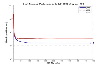
The mean square error from the training set decreases with the number of epochs whilst the error on the validation set decreases up to epoch 50, and then increases relative to the training set. In this case, the early stopping criterion was not satisfied since the validation error remained relatively consistent through this training run. Overall, we achieved a training accuracy of 98.5%. Although the cross-entropy “performance” metric is preferred for this type of problem, both the mean square error and cross entropy performance metrics gave identical values (0.0184).
Test set evaluation
In our case, the recall rate is of special interest because we want to mitigate the effect of misclassifying people as “not left”. As such, we set the focus on comparing the two test set results based on their recall rates. The confusion matrix for SVM and MLP are shown in the left and right plots below.
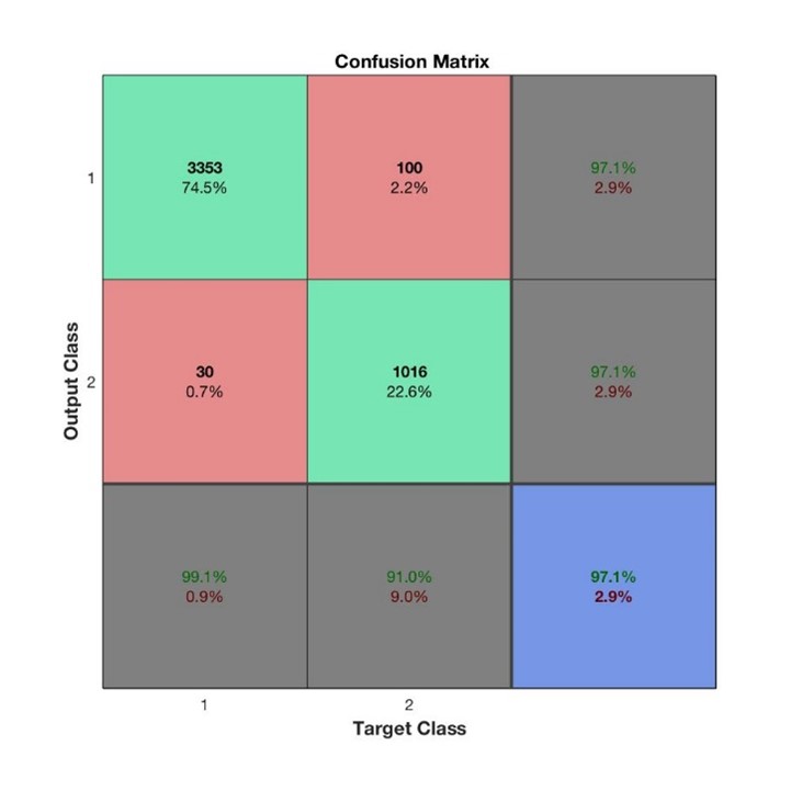

SVM resulted in a recall rate of 91% whilst MLP led to 93.3%, an important improvement. For precision, we can see the reverse effect with a precision rate of 97.1% for SVM vs 93.8% for MLP. The final test set accuracy scores can also be observed in the confusion matrices (in the blue square) and shows that in terms of accuracy, SVM is better with 97.1% compared to MLP of 96.8%.
Conclusion
In essence, both algorithms accomplished a very high and comparable performance on this data set to classify employee departure. For the choice of HP in this experiment, the training time was a big issue for both SVM and MLP. Splitting the hyperparameter search of SVM into two phases was an important decision to reduce the compute time. An alternative way of evaluating if a Gaussian kernel might be more suitable than a linear kernel could be done through investigating a 2D PCA plot. If the decision boundary is highly non-linear, we could have ruled out the linear kernel right from the beginning and saved some time tuning over different kernel functions. The second tuning round, on a random grid with only 10 individual combinations of values on 5-fold cross validation, took around 2 hours. In the end, random search did not find any better values for σ and C but this is only due to the fact, the restricted the random search procedure to only 10 random combinations. A larger number of combinations would probably result in even better HP compared to the default values, which were better than the random values found by the tuning process. However, considering that computational power was limited, this was not possible for us to explore. We also evaluated our results in Python using Sci-kit learn [13] and found that tuning was much faster compared to the MATLAB implementation. HP tuning has an even greater effect on MLP compared to SVM due to the wider range of parameters that can be tuned. In addition, the choice of backpropagation algorithm during the tuning process can make a huge difference to training time. The SCG method implemented here takes approximately 30 seconds for tuning one set of HP (including 5-fold cross validation). For the 12 combinations in this experiment, this took approximately 6 minutes. In contrast, BR took around 10 minutes for training one run of the optimally tuned HP on the training dataset. Although BR gives more accurate results, it would have taken around 6 hours if used for tuning instead of SCG, which is not practical.
In terms of the final results, we are not surprised that MLP had a higher recall rate compared to SVM. Reducing false negatives has a great importance for this kind of problem set as we do not want to overlook key employees leaving the company. We suppose that the capabilities of learning higher level features through its hidden layers and non-linear activations are what gave it an edge compared to SVM. A limitation of our study was that we were not able to test the effect of momentum as one of our tuning parameters since it is not implemented in the BR algorithm chosen for this study. Momentum usually allows faster convergence and prevents a network from getting stuck in a local minimum [6] [9].
References
- [1] Bergstra, J., & Bengio, Y. (2012). Random search for hyper-parameter optimization. Journal of Machine Learning Research, 13(Feb), 281-305.
- [2] Caruana, R., Lawrence, S. and Giles, L., 2000, November. Overfitting in neural nets: Backpropagation, conjugate gradient, and early stopping. In NIPS (pp. 402-408).
- [3] Chawla, N.V., Bowyer, K.W., Hall, L.O. and Kegelmeyer, W.P., 2002. SMOTE: synthetic minority over-sampling technique. Journal of artificial intelligence research, 16, pp.321-357.
- [4] Description of MLP algorithm and diagram in Scikit-learn http://scikit- learn.org/stable/modules/neural_networks_supervised.html
- [5] Foresee, F.D. and Hagan, M.T., 1997, June. Gauss-Newton approximation to Bayesian learning. In Neural Networks, 1997., International Conference on (Vol. 3, pp. 1930-1935). IEEE.
- [6] Haykin, S. S., 1999, Neural networks: a comprehensive foundation, 2nd edn, Prentice Hall, Upper Saddle River, N.J.
- [7] Kaggle dataset, https://www.kaggle.com/ludobenistant/hr-analytics
- [8] MacKay, D.J., 1992. Bayesian interpolation. Neural computation, 4(3), pp.415-447.
- [9] MATLAB Neural Network Toolbox Documentation, https://uk.mathworks.com/help/nnet/
- [10] MATLAB Statistics and Machine Learning Toolbox, https://uk.mathworks.com/products/statistics.html
- [11] Møller, M.F., 1993. A scaled conjugate gradient algorithm for fast supervised learning. Neural networks, 6(4), pp.525-533.
- [12] Ng, Andrew, 2015, CS229 Machine Learning lecture note 3, from: http://cs229.stanford.edu/materials.html accessed March 2017
- [13] Pedregosa, F., Varoquaux, G., Gramfort, A., Michel, V., Thirion, B., Grisel, O., Blondel, M., Prettenhofer, P., Weiss, R., Dubourg, V. and Vanderplas, J., 2011. Scikit-learn: Machine learning in Python. Journal of Machine Learning Research, 12(Oct), pp.2825-2830.
Comments powered by Disqus.