Using Advanced Regression Techniques to Predict House Prices

In this example, we will use the Ames, Iowa Housing dataset from Kaggle to fit a model to predict the final price of each house using the 79 explanatory variables in the dataset [1]. The code for this exercise can also be accessed from github. Download the train.csv and test.csv from the Kaggle website and store and read the data into a pandas dataframe replacing the path depending on where it is stored.

import pandas as pd
train = pd.read_csv(<path to train.csv>)
test = pd.read_csv(<path to test.csv>) 
test.head(5)

	Id	MSSubClass	MSZoning	LotFrontage	LotArea	Street	Alley	LotShape	LandContour	Utilities	…	ScreenPorch	PoolArea	PoolQC	Fence	MiscFeature	MiscVal	MoSold	YrSold	SaleType	SaleCondition
0	1461	20	RH	80.0	11622	Pave	NaN	Reg	Lvl	AllPub	….	120	0	NaN	MnPrv	NaN	0	6	2010	WD	Normal
1	1462	20	RL	81.0	14267	Pave	NaN	IR1	Lvl	AllPub	….	0	0	NaN	NaN	Gar2	12500	6	2010	WD	Normal
2	1463	60	RL	74.0	13830	Pave	NaN	IR1	Lvl	AllPub	…	0	0	NaN		MnPrv	NaN	0	3	2010	WD	Normal
3	1464	60	RL	78.0	9978	Pave	NaN	IR1	Lvl	AllPub	…	0	0	NaN		NaN	NaN	0	6	2010	WD	Normal
4	1465	120	RL	43.0	5005	Pave	NaN	IR1	HLS	AllPub …	144	0	NaN	NaN	NaN	0	1	2010	WD	Normal

Some of the columns in the training dataset seem to have a lot of missing values. It would be sensible to drop these columns if the number of missing values comprises more than some threshold (say 15%) of the data in the column.

frac = train.shape[0]*0.9 # number of non NA values we are satisfied with in each column . Lets say we need at least 90% non-NA values (columns with more than these will be dropped)
percent_missing = (100*(train.isnull().sum())/train.shape[0]).round(1) 
percent_missing.sort_values(ascending = False).head(20)

'''
PoolQC          99.5
MiscFeature     96.3
Alley           93.8
Fence           80.8
FireplaceQu     47.3
LotFrontage     17.7
GarageCond       5.5
GarageType       5.5
GarageYrBlt      5.5
GarageFinish     5.5
GarageQual       5.5
BsmtExposure     2.6
BsmtFinType2     2.6
BsmtFinType1     2.5
BsmtCond         2.5
BsmtQual         2.5
MasVnrArea       0.5
MasVnrType       0.5
Electrical       0.1
Utilities        0.0
dtype: float64
'''

We can see certain variables PoolQC, MiscFeature, Alley, Fence, FireplaceQu with a high proportion of missing values. Variables concerning Garage and Basmement also account for less than 5% missing values. We need to inspect these categorical variables in more detail to determine if these are indeed ‘missing values’ or labelled NaN because of an absence of a feature eg. garage, fence, alley etc.For the latter case, we need to set the NaN values to ‘None’.

Grouping all categorical variables with NaN values. Variables belonging to similar categories have been grouped together for comparison e.g. Basement, MasVnr, Garage etc. Non-categorical variables have also been included (e.g Pool Area, MasVnrArea) if they help in deciding if the NaN in categorical variable of the same category need to be set to None or dropped. If PoolQC is NaN and PoolArea is 0 it is highly likely that the NaN means an absence of a pool and should be said to None.

train_cat = train[['BsmtFinType1','BsmtFinType2','BsmtCond', 'BsmtQual','Electrical','MasVnrArea','MasVnrType', 
                   'GarageCond','GarageFinish','GarageQual','GarageType','GarageYrBlt','MiscFeature','Fence',
                   'PoolQC','PoolArea','Alley','FireplaceQu']]

train_cat.head(5)

The table above shows that NaN values of all variables should be set to ‘None’. Garage variables : Where there are NaN values, they occur in all garage variables suggesting absence of garages for those houses Pool - PoolQC is set to NaN corresponding to PoolArea of 0, suggesting absence of Pool. This should be set to ‘None’ Basement : Similarly, NaN values in Alley, Fence, Miscfeatures suggest absence of this feature in the house and should be set to ‘None’ In case of the Electrical variable, setting the NaN value to ‘None’ does not make sense as it is a feature that all houses should have. Since it only accounts for 0.1% of the observations,the corresponding rows will be dropped.

Categories = ['BsmtFinType1','BsmtFinType2','BsmtCond', 'BsmtQual','MasVnrType', 'GarageCond','GarageFinish',
              'GarageQual','GarageType','GarageYrBlt','MiscFeature','FireplaceQu','Fence','PoolQC','Alley']
train[Categories] = train[Categories].replace(np.nan, 'None', inplace = True)

We now need to impute missing values for the non-categorical variable using the mean of each univariate distribution. The catgeorical variables will then be one hot encoded to covert into numbers for furthr analysis (correlation/ modelling).

import pandas as pd
from sklearn import preprocessing 
Noncat = ['LotFrontage','MasVnrArea']
imp = preprocessing.Imputer(missing_values='NaN', copy = False, strategy='mean', axis=0)
imp.fit(train[Noncat])

train= pd.get_dummies(data=train) 

Feature Engineering

Now we will determine which features are important for subsequent analysis and must be inlcuded. We will first calculate the correlation of all variables with sales price and filter out variables which correlate less than abs 0.5.Using these filtered features we will then create a correltion matrix to determine which of these features display multicollinerity with other dependent variables. Similar features can either be merged into one compound feature or just one of th features included in subsequent analysis

import numpy as np
import pandas as pd

corr1 = train.corr()['SalePrice'] 
corr =corr1[np.abs(corr1) > 0.5]  
corr = pd.DataFrame(data=corr,columns= ['SalePrice'])
corr = corr.drop_duplicates().sort_values('SalePrice',ascending =False)

	SalePrice
SalePrice	1.000000
OverallQual	0.790982
GrLivArea	0.708624
GarageCars	0.640409
GarageArea	0.623431
TotalBsmtSF	0.613581
1stFlrSF	0.605852
FullBath	0.560664
TotRmsAbvGrd	0.533723
YearBuilt	0.522897
YearRemodAdd	0.507101
KitchenQual_Ex	0.504094
KitchenQual_TA	-0.519298
ExterQual_TA	-0.589044

We can see that the Overall Quality and Garage Living area showed strong positive correlation with sale price. Other variables which showed > 50% correlation with sales price were:GarageCars,GarageArea, TotalBsmtSF, 1stFlrSF,FullBath,TotRmsAbvGrd,YearBuilt,KitchenQual_TA and ExternalQual_TA.

The KitchenQual_TA and ExternalQual_TA dummy variables which correspond to normal/average quality of kitchnen and exterior showed some negative correlation (< -0.6%) with sales price which is what one would expect i.e. as house price increases the quality of kitchen and exterion should become ‘less average’ and vice versa We will now plot a new correlation matrix with these filtered variables.

import matplotlib.pyplot as plt 
import seaborn as sns
corr_var = ['OverallQual','GrLivArea', 'GarageCars', 'GarageArea','TotalBsmtSF', '1stFlrSF', 'FullBath', 
            'TotRmsAbvGrd', 'YearBuilt','KitchenQual_TA', 'ExterQual_TA','SalePrice']
train = train[corr_var]
corr_matrix = train.corr()
f,ax = plt.subplots(figsize =(10,10))
sns.heatmap(corr_matrix, vmax=1,square=True)

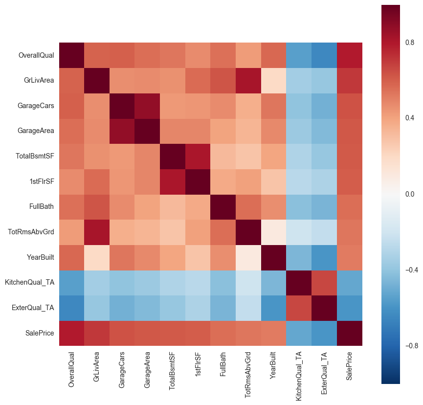
We find similar variables correlating with each other e.g. GarageCars and GarageArea, 1stFlrSF and TotalBsmtSF, GLivArea and TotRmsAbvGrd, Kitchen/external_Qual shows some correlation with the overall quality (compound variable) and year built. So we can drop one of the variables which show multicollinearity. Here GarageArea, TotalRmsAbvGrd,1stFlrSF, KitchenQual, ExternalQual were dropped because they correlated less with sales price compare to the other variables they correlated with.

labels_to_drop = ['GarageArea','TotRmsAbvGrd','1stFlrSF', 'KitchenQual_TA','ExterQual_TA']
train = train.drop(labels_to_drop, axis =1)
train.head(10) 

	OverallQual	GrLivArea	GarageCars	TotalBsmtSF	FullBath	YearBuilt	SalePrice
0	7	1710	2	856	2	2003	208500
1	6	1262	2	1262	2	1976	181500
2	7	1786	2	920	2	2001	223500
3	7	1717	3	756	1	1915	140000
4	8	2198	3	1145	2	2000	250000
5	5	1362	2	796	1	1993	143000
6	8	1694	2	1686	2	2004	307000
7	7	2090	2	1107	2	1973	200000
8	7	1774	2	952	2	1931	129900
9	5	1077	1	991	1	1939	118000

We have now got a dataframe with the SalePrice (output variable) and 6 predictor variables. Now we need to process the data further for outliers

Outlier Detection

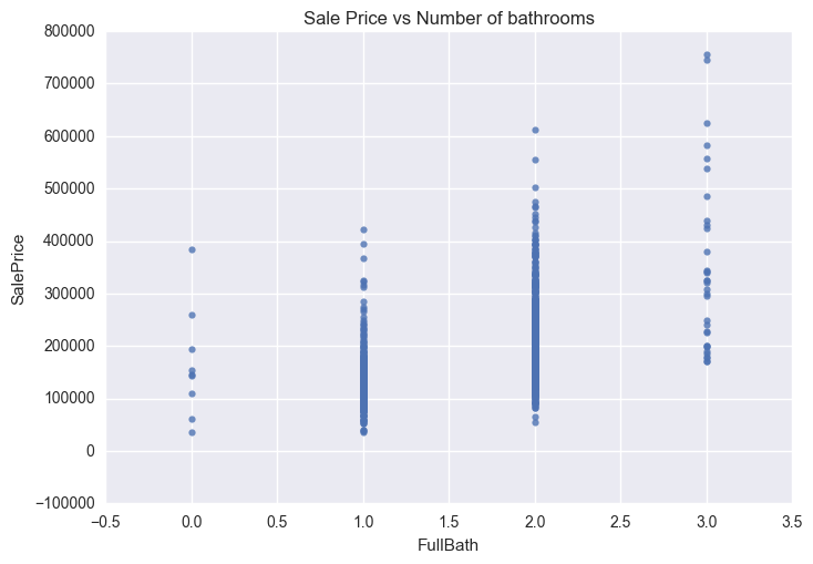
Most commonly used method to detect outliers is visualization like Box-plot, Histogram, Scatter Plot. Here I will use scatter plots for the continous variables and boxplots for the categorical variables. We can use certain rules of thumb like: Any value, which is beyond the range of -1.5 x IQR to 1.5 x IQR Data points, three or more standard deviation away from mean If a few isolated points lie outside the general trend line, then they can be deleted.

import seaborn as sns
import matplotlib.pyplot as plt 
%matplotlib inline

plt.figure()
sns.set(color_codes=True)
ax = sns.regplot(x="GrLivArea", y="SalePrice", data=train)
plt.title('Sale Price vs Ground Living Area')

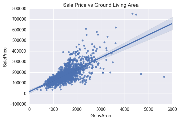
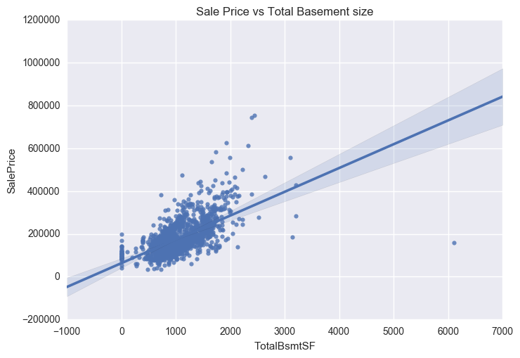
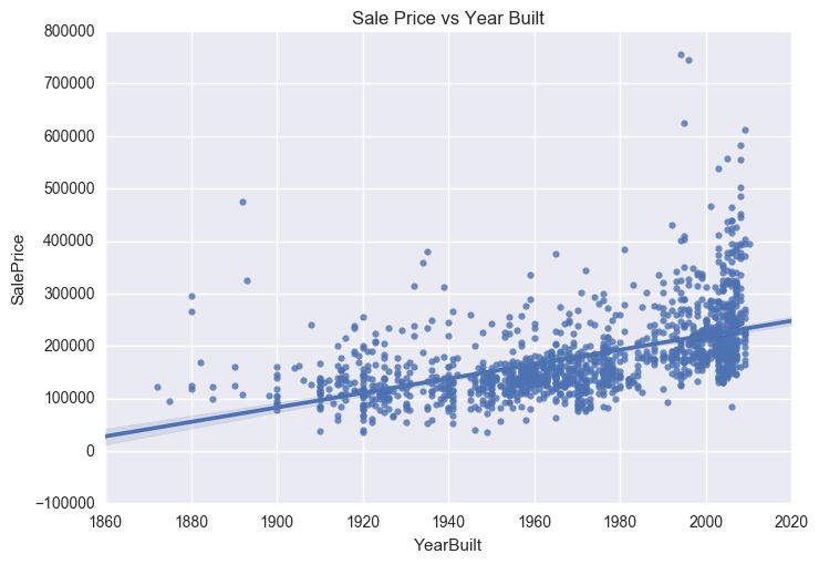
Four outliers in the graphs above will be dropped. These corresponding to GrLivArea > 4500 and SalePrice between 7000 and 8000 in the Sale Price vs Year Built graph. The isolated point in the Sale Price vs Total Basement Size graph, corresponding to TotalBsmtSF > 6000 will also be removed.

train =train.drop(train[train.GrLivArea == 5642].index)
train =train.drop(train[train.GrLivArea == 4476].index)
train =train.drop(train[train.SalePrice == 755000].index)
train =train.drop(train[train.SalePrice == 745000].index)

Standardisation of datasets

Standardisation is a common requirement for most sklearn estimators. Features in dataset need to follow a normal distribution (zero mean and unit variance). If this is not the case, then the models will perform badly [2].

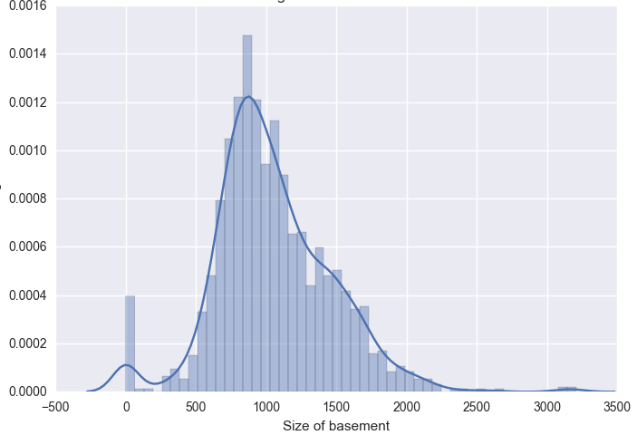
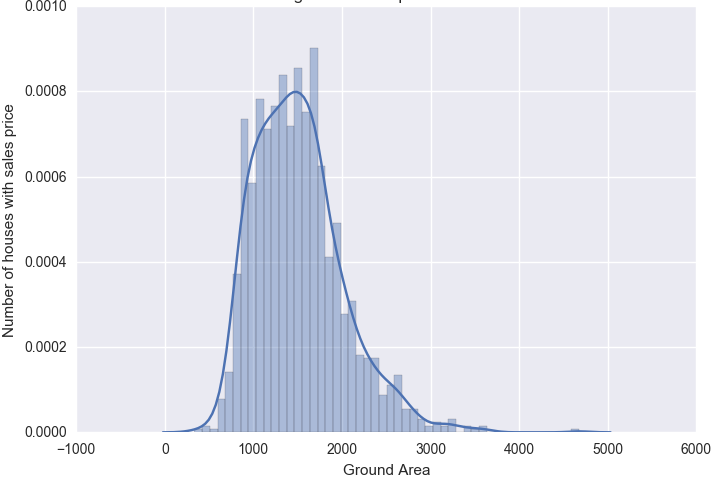
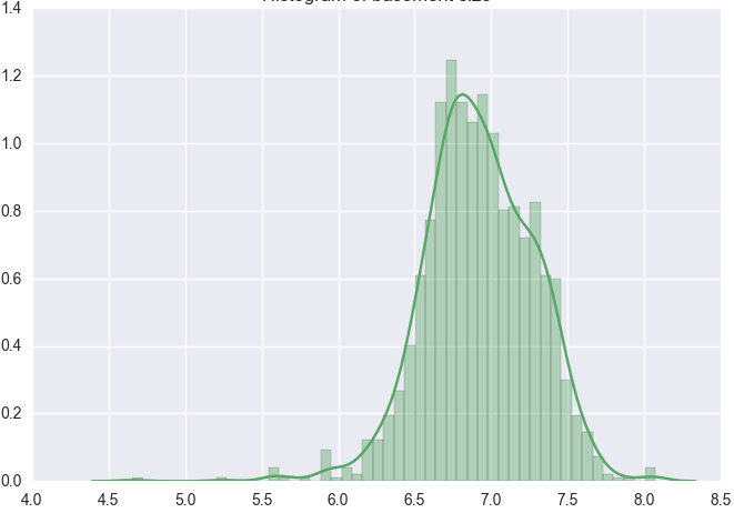
Lets look at the distribution of some of the continuos variables like TotalBsmtSF and GrLivArea using seaborn.distplot() function.

We can also use scipy.stats.probplot to generate a probability plot of feature against the quantiles of normal distribution [3]. For example use the code block below to generate a normal probability plot for GrLivArea. A straight, diagonal line indicates normally distributed data. However, in this case, there is positive skew which indicates non-normality.

from scipy import stats
stats.probplot(df_train['GrLivArea'], plot=plt)

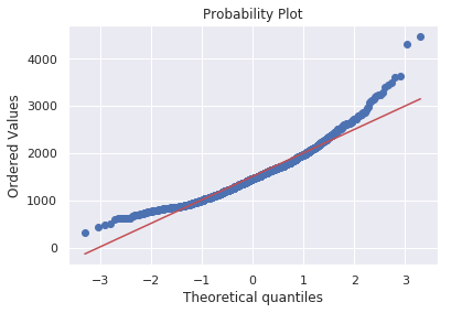
Since distributions above are skewed, the data needs to be standardised to make them normally distributed. One way of doing this is by removing the mean value of each feature, then scale it by dividing non-constant features by their standard deviation [2]. Alternatively, a log transformation can be applied althought it can’t be applied to zero or negative values. The histogram above also shows some zero values for basement size which would not be suitable for log transformation unless they are removed.

We can do this using the code block below. This will log transform the histogram of ground living area.

import numpy as np 
import matplotlib.pyplot as plt 
import seaborn as sns

train_new = train.drop(train[train['TotalBsmtSF']==0].index, axis =0)

train_new.loc[:,['SalePrice','TotalBsmtSF','GrLivArea','YearBuilt']] = np.log(train_new[['SalePrice','TotalBsmtSF','GrLivArea','YearBuilt']])

plt.figure()
sns.set(color_codes=True)
ax = sns.regplot(x="GrLivArea", y="SalePrice", data=train_new)
plt.title('Log Sale Price vs Log Ground Living Area')

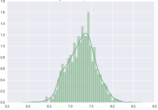
The distribution is now centred and more normally distributed and less skewed.

Similarly we can do the same for the other histograms for TotalBsmtSF.

We also need to treat heteroskedasticity i.e. dependent variable(s) exhibit unequal levels of variance across the range of predictor variable. This normally manifests as a cone-like shape in a scatterplot between the two variables, as the scatter (or variability) of the dependent variable widens or narrows as the value of the independent variable increases. This is evident in the scatter plots of SalePrice vs TotalBsmtSF and GrLivArea shown previously, where there is a larger dispersion on one side of the graph compared to the other.

Lets now generate the same plots following log transformation.

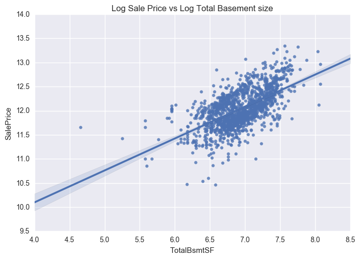
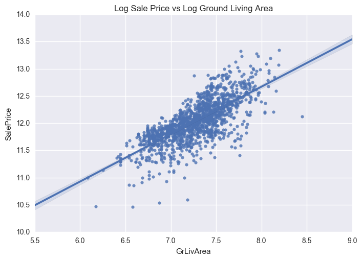
We can now see that the dense clutter in the scatter plots are now shifted towards the centre following log transformation. As a result, the data will exhibit less heteroskedasticity (absence of the conical shape like in the previous plots).

Now lets apply all the pre-processing tasks above to the test data. We can directly keep the same features in the test set as we did in the training set. We can then check if we need to replace any missing values. We will not need to create any dummy variables as all categorical variables were removed after correlation analysis.

var = ['OverallQual','GrLivArea', 'GarageCars','TotalBsmtSF', 'FullBath','YearBuilt']

test_id = test[['Id']] 
test = test[var]

test['GarageCars'] = test['GarageCars'].fillna((test['GarageCars'].mean()))
test['TotalBsmtSF'] = test['TotalBsmtSF'].fillna((test['TotalBsmtSF'].mean()))

# taking log transform 
test[['TotalBsmtSF']] = test[['TotalBsmtSF']].replace(0,1)

test.loc[:,['TotalBsmtSF','GrLivArea', 'YearBuilt']] = np.log(test[['TotalBsmtSF','GrLivArea','YearBuilt']])

Our test data is now ready for testing our model on once we have trained it on the training dataset

Modelling

Since the fit() method of scikit-learn estimator, expects the features and target variables to be passed in as separate arrays, we will create the train_x and train_y objects containing only the features and response variable respectively.

train_y = train_new['SalePrice']  
train_x = train_new.drop('SalePrice', axis =1)

	OverallQual	GrLivArea	GarageCars	TotalBsmtSF	FullBath	YearBuilt
0	7	7.444249	2	6.752270	2	7.602401
1	6	7.140453	2	7.140453	2	7.588830
2	7	7.487734	2	6.824374	2	7.601402
3	7	7.448334	3	6.628041	1	7.557473
4	8	7.695303	3	7.043160	2	7.600902
5	5	7.216709	2	6.679599	1	7.597396
6	8	7.434848	2	7.430114	2	7.602900
7	7	7.644919	2	7.009409	2	7.587311
8	7	7.480992	2	6.858565	2	7.565793
9	5	6.981935	1	6.898715	” 1	7.569928

We will now try a number of models to solve the regression problem. These include the following:

Ridge regression: addresses some of the problems of Ordinary Least Squares by imposing a penalty on the size of coefficients. The ridge coefficients minimize a penalized residual sum of squares

• Lasso Regression: estimates sparse coefficients. It is useful in some contexts due to its tendency to prefer solutions with fewer parameter values, effectively reducing the number of variables upon which the given solution is dependent.

• Support Vector Machines: The Support Vector Regression (SVR) uses the same principles as the SVM for classification, with only a few minor differences. In the case of regression, a margin of tolerance (epsilon) is set. The goal is to find an optimal hyperplane that deviates from yn by a value no greater than epsilon for each training point x, and at the same time is as flat as possible.The free parameters in the model are C and epsilon.

• Gradient Boosting (GB) Regressor: GB builds an additive model in a forward stage-wise fashion; it allows for the optimization of arbitrary differentiable loss functions. In each stage a regression tree is fit on the negative gradient of the given loss function.

We use 10 fold cross validation and r2 for the cross validation score for each fold. The metric is then reported as an average over all folds.

from sklearn.cross_validation import cross_val_score,cross_val_predict,StratifiedKFold
from sklearn import linear_model, svm
from sklearn.ensemble import GradientBoostingRegressor as xgb 
from sklearn.metrics import confusion_matrix,accuracy_score,f1_score
from sklearn import preprocessing 

# Ridge Regression 

clf_Ridge = linear_model.Ridge(fit_intercept=True, normalize=True, alpha = 0.01) 
clf_Ridge.fit(train_x, train_y)  
clf_Ridge_score = cross_val_score(clf_Ridge,train_x, train_y, cv = 10, scoring = 'r2')

# Support Vector Regression 
X_scaler = preprocessing.StandardScaler()
train_x = X_scaler.fit_transform(train_x)
clf_SVR = svm.SVR(kernel='rbf', gamma='auto',C = 1,epsilon = 0.1)
clf_SVR.fit(train_x, train_y)
clf_SVR_score = cross_val_score(clf_SVR, train_x, train_y, cv = 10, scoring='r2') 

# LassoCV

clf_lasso = linear_model.LassoCV()
clf_lasso.fit(train_x, train_y)
clf_lasso_score = cross_val_score(clf_lasso, train_x, train_y, cv = 10, scoring='r2') 

# Gradient Boosting Regressor 

clf_xgb = xgb(learning_rate=0.01, n_estimators=500, max_depth=3, subsample= 0.5)
clf_xgb.fit(train_x, train_y)
clf_xgb_score = cross_val_score(clf_xgb, train_x, train_y, cv = 10, scoring='r2') 

# R squared coefficients for all the models after training 

print ("")
print("The R2 score using for Ridge is %f" % (clf_Ridge_score.mean()))
print("The R2 score for Lasso is %f" % (clf_lasso_score.mean())) 
print("The R2 score for SVR is %f" % (clf_SVR_score.mean())) 
print("The R2 score for Gradient Boosting Regression is %f" % (clf_xgb_score.mean())) 


'''
The R2 score using for Ridge is 0.825067
The R2 score for Lasso is 0.825010
The R2 score for SVR is 0.826482
The R2 score for Gradient Boosting Regression is 0.834290
'''

The Gradient Boosting Regression had the highest R2 score (0.834) followed by the SVR (0.826) We can now use the Gradient Boosting Regression model to generate predictions on unseen data. However, before doing this we need to re-apply the transformation to test set, using the mean and standard deviation computed previously on the training dataset. We then need to calculate the exponent of the results, as data is in log scale.

import numpy as np
import pandas as pd 

test_x = X_scaler.transform(test)
predict = pd.DataFrame(np.exp(clf_xgb.predict(test_x)), columns= ['SalePrice'])  

References

1 Dataset Source https://www.kaggle.com/c/house-prices-advanced-regression-techniques/data 2 Preprocessing Data sklearn doc https://scikit-learn.org/stable/modules/preprocessing.html

1. Scipy Probability Plot doc https://docs.scipy.org/doc/scipy/reference/generated/scipy.stats.probplot.html