
Measuring wellbeing of a population is important to understand what factors affect individuals in their daily lives. Poor wellbeing can lead to a number of mental health problems, which can result in unnecessary visits to the hospital and a severe reduction in the quality of life and inability to carry out daily tasks with full efficiency. Local authorities in London rely on wellbeing data in order to target resources, and with local authorities currently gaining more responsibilities from government, this is of increasing importance [1]. The insights about wellbeing could help provide a firm evidence base for informed local policy-making, and justify the distribution of regeneration funds. In addition, it could identify causes behind improvements in wellbeing in certain areas, which could help in policy decision making.
We will explore a dataset from the London Datastore [2] which contains a wealth of information regarding wellbeing scores and factorswhich contribute to wellbeing across 625 London wards. These wellbeing scores present a combined measure of wellbeing indicators of the resident population based on different factors such as health, childhood obesity, incapacity benefits claimant rate, economic security, safety, education, children, families, transport, environment and happiness. Each of these indicators is subdivided into further categories resulting in 76 attributes in the dataset.
For the majority of this analysis, only the 2011 wellbeing scores were used as this would give a larger variable pool after merging with the ‘census 2011’ and ‘access to open space’ datasets [2]. Since most counts were represented as a percentage of the total population in the dataset, no normalisation was required. However, a z-score transformation was applied to scale the range of the variables before Geographically Weighted Regression (GWR) modelling. The aim is to identify the most discriminating and generalisable socio-economic variables that appear to drive spatial differences using information published by the Office for National Statistics (ONS) [3] and other government and public health organisations. This lead to the formulation of the following questions:
- How did wellbeing scores vary across London in 2011 and how did they compare to 2010 and 2012?
- Which factors had the most impact on wellbeing scores across London in 2011 and do the relationships with wellbeing exhibit any non-stationarity which can be modelled effectively?
We can visually inspect how 2011 wellbeing scores vary spatially across London wards by plotting the raw scores on Choropleth maps.
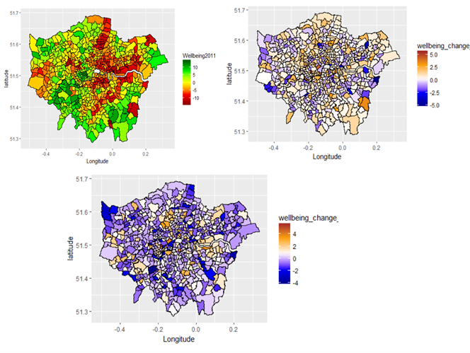
The top left map shows wards with positive(green) and negative(red) wellbeing scores. Poor wellbeing seems to associated with wards along the stretch from north to south (through central London) and parts of the east. The top right and bottom maps show a change in wellbeing scores in 2010 and 2012 respectively, calculated relative to wellbeing scores in 2011. Wellbeing scores in 2012(figure c) got progressively worse in wards outside Central London compared to 2011. In 2010, a larger proportion of wards in London had better wellbeing scores relative to 2011, with few wards on the outskirts and central London showing worse wellbeing scores.
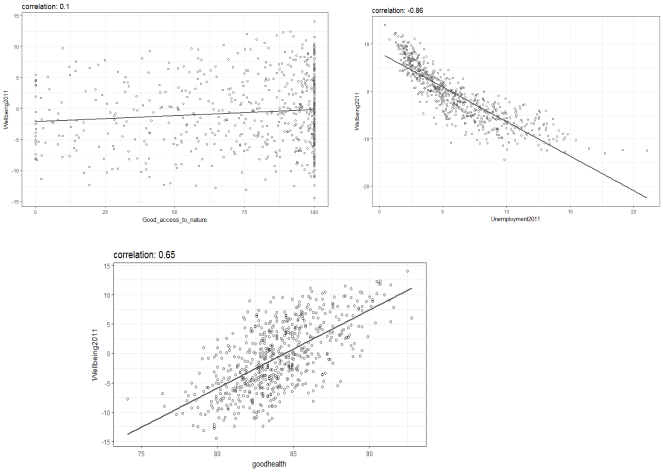
Scatter plots and Pearson Correlation coefficients can be used to investigate each variable’s relationship with wellbeing as shown below. Good health and unemployment show positive (correlation:0.65) and strong negative correlation (correlation: -0.86) respectively with wellbeing but surprisingly, good access to nature showed no significant correlation to wellbeing. Variables with poor correlation were removed from subsequent analysis. The only exception being the happiness score (correlation:0.3), as publications from the ONS deemed this factor to be very important for determining subjective wellbeing.
The correlation between the selected variables was investigated further by computing a correlation matrix as in plot below. We can see that variables which correlate strongly with wellbeing also correlate strongly with many other variables.
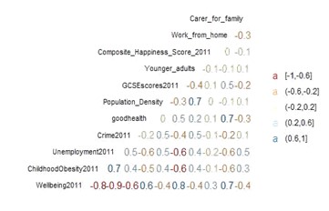
This problem of collinearity was investigated further by computing VIF scores [7,11]. The table below summarises the VIF scores generated for each of these variables and how these scores reduced after removing four variables. This results in final 10 variables which will be used for the modelling tasks.
| Variable | VIF_scores before | VIF_scores after |
| School_Absence | 2.2 | - |
| Life_Expectancy | 2.5 | - |
| Childhood_obesity | 2.4 | 2.1 |
| Population Density | 3.1 | 2.4 |
| Happiness_Score | 1.1 | 1.1 |
| Crime | 1.6 | 1.6 |
| GCSE_scores | 2.1 | 1.8 |
| good_health | 5.4 | 3.4 |
| Unemployment | 5.2 | 3.6 |
| Professionals | 10.5 | - |
| Younger_adults | 5.5 | 3.4 |
| Work_from_home | 5.3 | 2.2 |
| Carer_for_family | 1.7 | 1.3 |
| dependent_children | 8.1 | - |
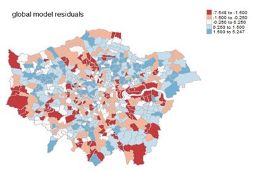
Using this smaller pool of variables, a refined multivariate regression model was fitted (R2= 0.92, p < 0.01). The residual plot shows some clusters of red and blue residuals in certain parts of London (north west and centre). Since we can see some spatial auto correlation of residuals, this suggests that another model is required which takes into account the spatial variation [9,11]. A fundamental element in GW modelling is that it quantifies the spatial relationship or spatial dependency between the observed variables and will hence be a good choice for the next steps in the analysis.
Modelling of the spatial relationships was achieved through a weighting function with Euclidean distance measure and a bisquare kernel function. The GWmodel package in R provides an option for automated bandwidth tuning for GWR, but not for GWSS [6,8]. Alternatively, the bandwidth can be manually chosen as shown in the example in figures below.
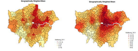
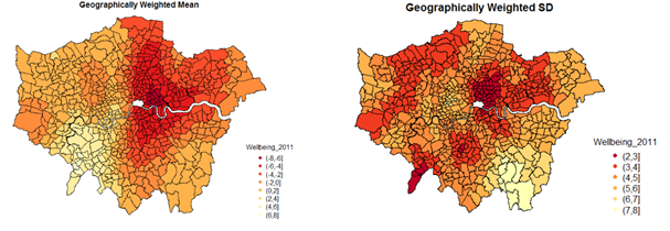
The smoothing effect increases with increasing bandwidth. The optimal bandwidth of 50 local points produced a dark red cluster in north and east-central side of London, a bright red pattern running from north to south and a bright yellow cluster in the south west. The GW standard deviation shows a high variation in wellbeing, concentrated in the south east.
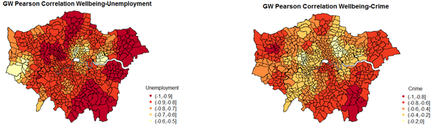
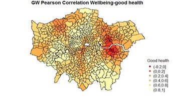
The GW correlation coefficients for unemployment, crime and good health (against wellbeing show that the strength of the relationships between these variables varies spatially. Unemployment and crime are both negatively correlated with wellbeing, but crime is more strongly correlated in the south-east wards and unemployment more so in the south, east and some wards in the north-west. Good health is positively correlated in most parts of London except for some wards in the east (red cluster).
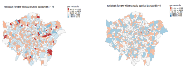
We now plot the residuals of the GWR model results for manually optimised bandwidth (50 local points) and auto tuned bandwidth (175 local points). The results of manual tuning (figure 6b) produced much smaller residuals across the whole of London compared to auto-tuning (figure 6a), where large negative residuals (dark red) can be seen in a number of wards. The results of auto-tuning produced similar pattern to the global model.
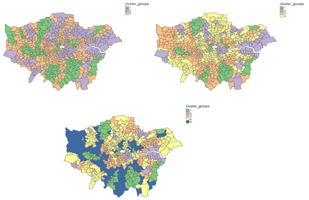
For the final analytical task, we explore how the explanatory variables vary spatially through k-means clustering on the geographically weighted regression coefficients [10]. This will allow identification of wards that share similar combinations of relationships. A z-score transformation is applied so no variable is preferentially weighted due to its range of values. A range of k values were used to generate clustering solutions. An example of clustering output using three, four and five clusters is shown in the left, right and bottom plots below. The four cluster solution produced the lowest withinness score. However, the pattern of clusters is not well defined and inconclusive with no distinct group of clusters.
Findings
The highest wellbeing scores were found in wards concentrated in the south west of London (Twickenham, Richmond park, Brentford, Ealing and Acton Central, Putney, Wimbledon, Chelsea etc.). This can be attributed to high levels of affluence in these areas, coupled with high levels of social cohesion. Concentrations of lower wellness scores (red coloured wards) were clustered around north and north-east London and some parts of the south and east London (Wards in between Oval, Crystal Palace, Woolwich, Lewisham). Additional clusters were also seen in more deprived areas in part of north-west London (Dollis Hill, Willesden) and along the outskirts on the west (Hayes and Harlington). The worst scores (dark red) being in wards of Upper Edmonton, Tottenham Hale, Bow East/West which have been known to be impoverished areas. Wellbeing scores got worse in many parts of London (more concentrated in the outskirts) in 2012 compared to 2011. In contrast, wellbeing was better in most wards around London (except for a few on the outskirts) in 2010 compared to 2011. This suggests that wellbeing was getting progressively worse every year. Economic and political events during that period may well have been a driving force behind these observations e.g. UK general election in 2010, recession in 2010.
The scatter plots and correlation matrix confirm that Unemployment correlated most strongly with wellbeing along with GCSE scores and Childhood Obesity. Surprisingly access to nature showed little or no correlated with wellbeing. Given the distribution of wellbeing scores across London, one would expect there to be a positive correlation as wards on the outskirts with large greenspaces and parks displayed higher wellbeing scores. Similarly, other explanatory variables like Transport deemed important for wellbeing, also showed no relationship, although people who worked from home showed better wellbeing.
The relationship between wellbeing and indicators exhibited non-stationarity. Residual plots from GWR and global model revealed that the spatial relationships between explanatory variables and wellbeing were best modelled using GWR with a manually tuning bandwidth of 40 local points. Thestrength of the correlation coefficients of variables spatially and in some cases the relationship with wellbeing was reversed e.g. good health was negatively correlated in boroughs of Greenwich and Newham.
Managing policy design requires us to measure wellbeing in different populations in different areas that may be affected by policy [13]. The chloropeth maps revealed an interesting pattern in geographically weighted mean wellbeing scores across London wards where wellbeing scores were lower in certain wards closer to north-central and east-central part of London, and higher in the southwest. The fact that the UK was plunged into a recession towards the autumn of 2010, may have been one of the driving factors behind the general worsening of wellbeing scores from 2010-2011 and 2011-2012. This also suggest that the policies in place during those years was not sufficient as populations in more areas of London were also expressing lower wellbeing. In contrast to results from the commonly used global regression model, geographically weighted regression showed that variables (unemployment, crime, education as examples) also influenced wellbeing scores to a different extent in different areas of London. This is important as it would allow the local authorities to build a strong case for programmes tackling certain issues like unemployment in the most affected areas. [1,13].
This analysis has a number of limitations which need to be made clear. The data in this report has been aggregated to ward level and would hide variation which is more local. Data availability for small areas is far more limited. Furthermore, wellbeing score metrics computed on the London Datastore [2] were only available at ward level, which limits use of more local variables even if they were available. The indicators on the London Datastore were used as a basis for choosing the variables. More specific factors like loneliness and mental health/depression which are difficult to quantify, can also have a drastic effect on wellbeing.
References
- [1] Spence, A., Powell, M. and Self, A., 2011. Developing a Framework for Understanding and Measuring National Well-being. Office for National Statistics at http://www. ons. gov. uk/ons/guidemethod/userguidance/well-being/publications/previous-publications/index. html (accessed 17 October 2013).
- [2] London Datastore: Official site providing free access to ward well-being data, Access to Public Open Space and Nature by Ward data and census data. from the Greater London Authority. Datasets used: https://data.london.gov.uk/dataset/london-ward-well-being-scores https://data.london.gov.uk/census/data/ https://data.london.gov.uk/dataset/access-public-open-space-and-nature-ward
- [3] Beaumont, J., 2011. Measuring national well-being: Discussion paper on domains and measures. Newport: Office for National Statistics.
- [4] Murray, D.G., 2013. Tableau Your Data!: Fast and Easy Visual Analysis with Tableau Software. John Wiley & Sons.
- [5] R Core Team., 2016. R: A language and environment for statistical computing. R Foundation for Statistical Computing, Vienna, Austria. URL https://www.R-project.org/
- [6] Gollini, I., Lu, B., Charlton, M., Brunsdon, C. and Harris, P. (2015), GWmodel: An R Package for Exploring Spatial Heterogeneity Using Geographically Weighted Models. Journal of Statistical Software, 63(17):1-50.
- [7] O’brien, R.M., 2007. A caution regarding rules of thumb for variance inflation factors. Quality & Quantity, 41(5), pp.673-690.
- [8] Brunsdon, C., Fotheringham, A.S. and Charlton, M., 2002. Geographically weighted summary statistics—a framework for localised exploratory data analysis. Computers, Environment and Urban Systems, 26(6), pp.501- 524.
- [9] Fotheringham, A.S., Brunsdon, C. and Charlton, M., 2003. Geographically weighted regression: the analysis of spatially varying relationships. John Wiley & Sons.
- [10] Jain, A.K., 2010. Data clustering: 50 years beyond K-means. Pattern recognition letters, 31(8), pp.651-666.
- [11] Wheeler, D. and Tiefelsdorf, M., 2005. Multicollinearity and correlation among local regression coefficients in geographically weighted regression. Journal of Geographical Systems, 7(2), pp.161-187.
- [12] Rousseeuw, P.J., 1987. Silhouettes: a graphical aid to the interpretation and validation of cluster analysis. Journal of computational and applied mathematics, 20, pp.53-65.
- [13] Hicks, S., Tinkler, L. and Allin, P., 2013. Measuring subjective well-being and its potential role in policy: Perspectives from the UK office for national statistics. Social Indicators Research, 114(1), pp.73-86.
- [14] Charlton, M., Brunsdon, C., Demsar, U., Harris, P. and Fotheringham, S., 2010. Principal components analysis: from global to local.
Comments powered by Disqus.