
Probabilistic Graphical Models (PGMs) are generative models that can compute the joint distribution among random variables in a system by explotiing the conditional indpendence relationship between variables to create a graph structure representing the relationships between different random variables. Graph structures can be directed, undirected or both and have a set of parameters associated with each variable (local conditional probabilities).
There are mainly 2 types of graphical models:
Markov Models: A Markov Models consists of an undirected graph and are parameterized by factors. Factors represent how much 2 or more variables agree with each other. Cycles are permitted in graphs e.g. Markov networks, Markov chains, HMM
Bayesian Models: A Bayesian Model consists of a directed and acyclic graph (DAG). Each node in the graph has local Conditional Probability Distributions(CPDs) to represent causual relationshp with other variables e.g. Discrete Bayesian Network, Continuous Bayesian Network, Dynamic BN, Bayesian Classifiers (Naive Bayes)
In the rest of this blog, we will be focussing only on Markov Models (Bayesian Models will be covered in a separate article).
Markov Chains
A Markov chain is a model that tells us something about the probabilities of sequences of random variables, states, each of which can take on values from some set. These sets can be words, or tags, or symbols representing anything, like the weather. A Markov chain makes a very strong assumption that if we want to predict the future in the sequence, all that matters is the current state. The states before the current state have no impact on the future except via the current state.
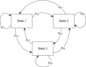
We can easily model a simple Markov chain with Python’s Pomegranate package and calculate the probability of any given sequence. We will consider a scenario of performing three activities: sleeping, running and eating. In the diagram above, each node will represent each of these states and the arrows determine the probability of that event occurring. We will assume the probabilities of transitioning from one state to another as in table below
| state1 | state2 | sequences |
|---|---|---|
| Sleep | Sleep | 0.10 |
| Sleep | Eat | 0.50 |
| Sleep | Run | 0.30 |
| Eat | Sleep | 0.10 |
| Eat | Eat | 0.40 |
| Eat | Run | 0.40 |
| Run | Sleep | 0.05 |
| Run | Eat | 0.45 |
| Run | Run | 0.45 |
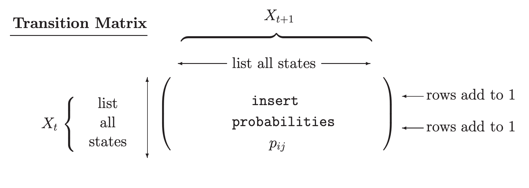
We also assume we have prior knowledge on probabilties of these activities occuring on average e.g. on a given day we sleep 50% of the time, eat 20% of the time and run 30% of the time. We can encode both the discrete distribution and the transition matrix in the MarkovChain class, as in the code block below
1
2
3
4
5
6
7
8
9
10
11
12
13
14
15
16
17
18
19
20
21
22
23
24
25
26
27
28
29
import numpy as np
import pandas as pd
from pomegranate import ConditionalProbabilityTable, DiscreteDistribution
import numpy as np

def initialise_markov_chain(prior_prob, cpd):
    d1 = DiscreteDistribution(prior_prob)
    d2 = ConditionalProbabilityTable(cpd, [d1])
    clf = MarkovChain([d1, d2])
    return clf

A = "Sleep"
B = "Eat"
C = "Run"

prior_prob = {A: 0.5, B: 0.2, C: 0.3}
cpd = [
    [A, A, 0.10],
    [A, B, 0.50],
    [A, C, 0.30],
    [B, A, 0.10],
    [B, B, 0.40],
    [B, C, 0.40],
    [C, A, 0.05],
    [C, B, 0.45],
    [C, C, 0.45],
]

clf = initialise_markov_chain(prior_prob, cpd)
Now, we can calculate the probability of any given sequence using the object returned from the code block above.
We can compute the probability of a given sequence of events e.g. “Run-Sleep-Eat-Sleep”. This will return a logarithm to handle small probability numbers.
1
2
3
4
5
6
def compute_probability_sequence(seq, clf):
    return clf.log_probability(seq)

compute_probability_sequence(['Run', 'Sleep', 'Eat', 'Sleep'], clf)]

# this gives -7.1954373514339185
Or perhaps we want to confirm that a sequence like “Sleep-Sleep-Eat-Sleep” has a higher likelihood.
1
2
3
compute_probability_sequence(['Sleep', 'Sleep', 'Eat', 'Sleep'], clf)

# -5.991464547107982
Now lets generate a random sample from the model with each observation sequence containing 4 events and we have 100 observed sequences in total.
1
2
3
4
5
6
7
8
9
10
import pandas as pd

def generate_random_sample_from_model(clf, length, num_seqs):
    df = pd.DataFrame(columns=["sequences"])
    for i in range(num_seqs):
        obs = clf.sample(length)
        df = df.append({"sequences": obs}, ignore_index=True)
    return df

df = generate_random_sample_from_model(clf, length=4, num_seqs=100)
the code block above outputs a dataframe as below, with each row in the sequences column containing a list of events which can be one of ‘Sleep’, ‘Eat’ or ‘Run’
| sequences | |
|---|---|
| 0 | [Run, Run, Run, Run] |
| 1 | [Eat, Eat, Eat, Eat] |
| 2 | [Sleep, Sleep, Eat, Sleep] |
| … | … |
| 98 | [Sleep, Eat, Run, Run] |
| 99 | [Sleep, Eat, Run, Run] |
We can then pass this as input to the MarkovChain.from_samples method. This expects the input to be a list of sequence lists.
1
2
3
4
5
6
7
8
9
10
11

from pomegranate import MarkovChain

def build_markov_chain_from_data(df):
    seq = list(df["sequences"])
    model = MarkovChain.from_samples(seq)
    return model

model_from_data = build_markov_chain_from_data(df)
print(model_from_data.distributions[1])
We can get the probabilities of all combinations of one state to another in a two event sequence. We can see that the probabilites estimated are very close to the original transition matrix.
| Eat | Eat | 0.4690265486725664 |
| Eat | Run | 0.4424778761061947 |
| Eat | Sleep | 0.08849557522123894 |
| Run | Eat | 0.4263565891472868 |
| Run | Run | 0.49612403100775193 |
| Run | Sleep | 0.07751937984496124 |
| Sleep | Eat | 0.5172413793103449 |
| Sleep | Run | 0.3620689655172414 |
| Sleep | Sleep | 0.12068965517241378 |
Hidden Markov Model
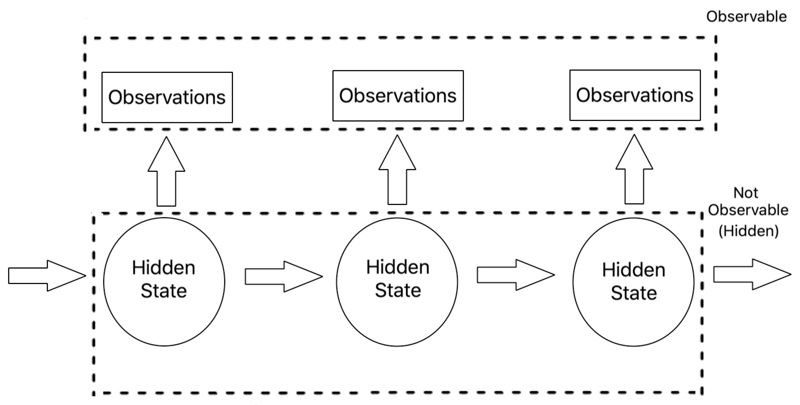
A Hidden Markov Models (HMM) are stochastic probabilistic models that aims to model a system as a Markov chain with hidden states and distinct transition and emission probabilities for each respective state. the nodes are hidden states which contain an observed emission distribution and edges contain the probability of transitioning from one hidden state to another. HMMs allow you to tag each observation in a variable length sequence with the most likely state according to the model.
When applying an HMM in the real world, there are three main subproblems that are associated with fitting the model.:
- Decoding : Given the model parameters and observed data, estimate the optimal sequence of hidden states.
- Likelihood: Given the model parameters and observed data, calculate the likelihood of the data.
- Learning: Given just the observed data, estimate the model parameters.
The first step can be solved by the dynamic programming algorithm known as the Viterbi algorithm This “decodes” the observation sequence to find the most probable sequence of hidden states. The Viterbi algorithm recursively computes the most probable path through a sequence of states by storing the probability and state sequence of the most probable path at each point in time (Viterbi 1967).
The second problem can be solved using the Forward-Backward algorithm. This recursively computes the forward probabilities which calculates the probability of ending in a state given the prior observation sequence (Baum and Eagon 1967). The algorithm does this by summing the probabilities of all the various hidden state paths that can potentially generate the observation sequence.
Finally, in order to estimate the model parameters, an iterative Expectation-Maximization algorithm known as Baum-Welch alogirthm which is used, which consists of two steps repeated until convergence.
- Use the available observed data of the dataset to estimate the missing data of the latent variables (Expectation Step). We now have the complete data.
- Using the complete data to update the values of the model parameters (Maximization Step)
1
2
3
4
5
6
7
8
9
10
11
12
13
14
15
16

def generate_random_sample_from_model(clf, length, num_seqs):
    df = pd.DataFrame(columns=["sequences"])
    for i in range(num_seqs):
        obs = clf.sample(length)
        df = df.append({"sequences": obs}, ignore_index=True)
    return df

def build_markov_chain_from_data(df):
    seq = list(df["sequences"])
    model = MarkovChain.from_samples(seq)
    return model

df = generate_random_sample_from_model(clf, length=4, num_seqs=100)
model_from_data = build_markov_chain_from_data(df)
print(model_from_data.distributions[1])
We can assign variables representing the different states, observations, transition and emission probability matrices, and generate a random sequence of observations. The input the fit() method in hmmlearn requires the input as a matrix of concatenated sequences of observations along with the lengths of the sequences. The code block below includes a helper function which returns concatenated array of sequences and an array of sequence lengths:
1
2
3
4
5
6
7
8
9
10
11
12
13
14
15
16
17
18
19
20
21
22
23
24
25
26
27
28
states = ["Rainy", "Sunny"]
n_states = len(states)
observations = ["walk", "shop", "clean"]
n_observations = len(observations)
start_probability = np.array([0.6, 0.4])
transition_probability = np.array([[0.7, 0.3], [0.4, 0.6]])
emission_probability = np.array([[0.1, 0.4, 0.5], [0.6, 0.3, 0.1]])

def generate_random_seq_of_observations():
    seq = deque()
    lengths = deque()
    for _ in range(100):
        length = random.randint(5, 10)
        lengths.append(length)
        for _ in range(length):
            r = random.random()
            if r < 0.2:
                seq.append(0)  # walk
            elif r < 0.6:
                seq.append(1)  # shop
            else:
                seq.append(2)  # clean
    seq = np.array([seq]).T
    return seq, lengths


seq, lengths = generate_random_seq_of_observations()
The EM algorithm training stops if the max number of iterations are reached or the change in score is lower than threshold tolerance set. We can monitor convergence by plotting the log likelihood per iteration. In this case, we have set the max number of iterations to 30.
1
2
3
4
5
6
7
8
9
10
11
12
13
14
15
16
17
18
19
20
21
22
23
24
25
26
27
28
29
30
31
32
33
34
35
36
37
38
39
40
41
42

def is_converged(hmm_model):
    return hmm_model.monitor_.converged


def train_discrete_hmm(
    X,
    lengths,
    start_probability,
    transition_probability,
    emission_probability,
    components=3,
    iterations=15,
    verbose=True,
):
    model = MultinomialHMM(components, iterations, verbose, init_params="mc")
    model.startprob_ = start_probability
    model.transmat_ = transition_probability
    model.emissionprob_ = emission_probability
    print(
        f"commencing hmm model training with parameters- "
        f"Iterations: {iterations}, components: {components}"
    )
    model.fit(X, lengths)
    if is_converged(model):
        print("model has converged")
        print(' ')
        print(model.transmat_)
        print(model.emissionprob_)
        print(model.startprob_)
    return model

model = train_discrete_hmm(
            seq,
            lengths,
            start_probability,
            transition_probability,
            emission_probability,
            components=n_states,
            iterations=30,
            verbose=True,
        )
Once we have the trained model, the inferred optimal hidden states can be obtained by calling predict method. The predict method can be specified with decoder algorithm (e.g virterbi or posterior estimation).
1
2
3
4
5
6
7
8
9
10
11
12
13
14
15

import numpy as np

def decode_hidden_state_for_discrete_hmm(encoded_obs_seq, observations, states, model):
    logprob, hidden_states = model.predict(encoded_obs_seq, algorithm="viterbi")
    print(
        "Observed behaviour:",
        ", ".join(map(lambda x: observations[x], encoded_obs_seq.T[0])),
    )
    print("Inferred hidden states:", ", ".join(map(lambda x: states[x], hidden_states)))
    return logprob, hidden_states

obs_states = np.array([[0, 2, 1, 1, 2, 0]]).T
decode_hidden_state_for_discrete_hmm(obs_states, observations, states, model)
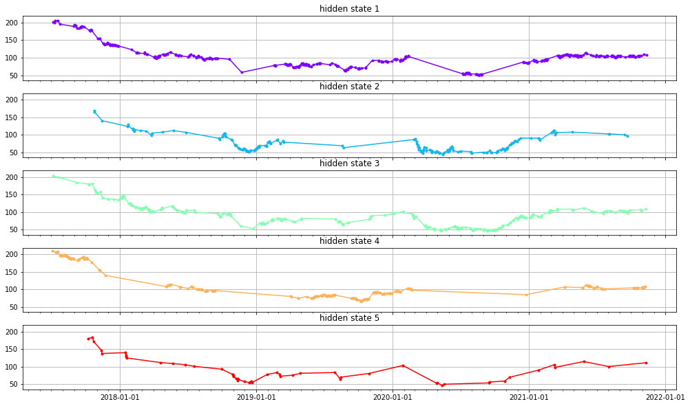
Regime Detection
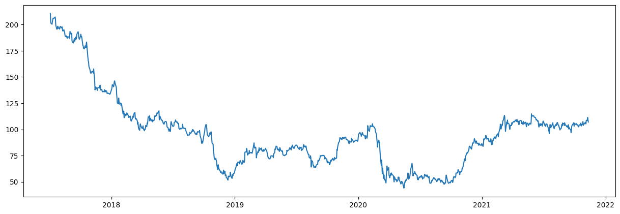
HMM can also be used for regime detection in time series stock data. Market conditions can change over time leading to up-beat (bullish) or down-beat (bearish) market sentiments (regimes). Because of the volatility in the data, it can be difficult to detect when (or even if) the bear market occurs. Since regimes of the total market are not observable, the modelling paradigm of hidden Markov model is introduced to capture the tendency of financial markets which change their behavior abruptly. Decoding the regimes can help in forecasting future market conditions
In this section we will fit a Gaussian HMM to yahoo stock market data and then decode the hidden states (regimes) from the observed returns We will use the Gaussian HMM interface from hmmlearn library on stock price data from Yahoo! finance.
Here the pandas_datareader library is used to fetch Yahoo Finance provides stock market data but has a rich source of stockd and shares data from various platforms.
1
2
3
4
5
6
7
8
9
10
11
12
13
14
15
16

import pandas_datareader.data as web
import datetime


def get_quotes_data_finance(start, end):

    Stocks = web.DataReader('GE', 'yahoo', start=start, end=end)
    Stocks.reset_index(inplace=True, drop=False)
    Stocks = Stocks.drop(["Open", "High", "Low", "Adj Close"], axis=1)
    return Stocks

start_date = datetime.date(2017, 7, 1)
end_date = datetime.datetime.now()

stocks = get_quotes_data_finance(start_date, end_date)
| Date | Close | Volume | |
|---|---|---|---|
| 0 | 2017-07-03 | 211.153839 | 2686450.0 |
| 1 | 2017-07-05 | 210.384613 | 2765126.0 |
| 2 | 2017-07-06 | 202.384613 | 9963967.0 |
| … | … | … | … |
| 1097 | 2021-11-09 | 111.290001 | 25123700.0 |
| 1098 | 2021-11-10 | 108.959999 | 8692600.0 |
| 1099 | 2021-11-11 | 107.000000 | 5504900.0 |
1
2
3
4
5
6
7
8
9
10
11
12
13
14
15
16
17
18
19
20
21
22
23
24
25
26
27
28
29

import numpy as np
import matplotlib.pyplot as plt

def preprocess_data(Stocks):
    Stocks = list(Stocks.itertuples(index=False, name=None))
    dates = np.array([q[0] for q in Stocks])
    end_val = np.array([q[1] for q in Stocks])
    volume = np.array([q[2] for q in Stocks])[1:]
    return dates, end_val, volume

def compute_end_val_delta(dates, end_val, volume):
    diff = np.diff(end_val)
    X = np.column_stack([diff, volume])
    return X

def plot_stocks_data(dates, end_val):
    plt.figure(figsize=(15, 5), dpi=100)
    plt.gca().xaxis.set_major_locator(YearLocator())
    plt.plot_date(dates, end_val, "-")
    plt.show()

dates, end_val, volume = preprocess_data(stocks)
X = compute_end_val_delta(dates, end_val, volume)
dates = dates[1:]
end_val = end_val[1:]
plot_stocks_data(dates, end_val)
plt.show()
1
2
3
4
5
6
7
8
9
10
11
12
13
14
15
16
17
18
19
20
21
22
23
24
25
26
27
28
29
30
31
32
33
34
35
36
37
38
39
40
import numpy as np
import pandas as pd
import matplotlib.cm as cm
import matplotlib.pyplot as plt
import numpy as np
from hmmlearn.hmm import GaussianHMM
from matplotlib.dates import MonthLocator, YearLocator


def train_gaussian_hmm(X, components, iterations):
    model = GaussianHMM(
        n_components=components, covariance_type="diag", n_iter=iterations, verbose=True
    ).fit(X)
    return model

def decode_hidden_states_time_series(X, model):
    hidden_states = model.predict(X)
    return hidden_states

def plot_trained_parameters(model, hidden_states, dates, end_val, figsize):
    fig, axs = plt.subplots(model.n_components, sharex=True, sharey=True, figsize=figsize)
    colours = cm.rainbow(np.linspace(0, 1, model.n_components))
    for i, (ax, colour) in enumerate(zip(axs, colours)):
        # Use fancy indexing to plot data in each state.
        mask = hidden_states == i
        ax.plot_date(dates[mask], end_val[mask], ".-", c=colour)
        ax.set_title(f"hidden state {i+1}")

        # Format the ticks.
        ax.xaxis.set_major_locator(YearLocator())
        ax.xaxis.set_minor_locator(MonthLocator())
        ax.grid(True)
    plt.show()

components=5
iterations=100000
model = train_gaussian_hmm(X, components,iterations)
hidden_states = decode_hidden_states_time_series(X, model)

plot_trained_parameters(model, hidden_states, dates, end_val, (17,10))
References
- Lawrence R. Rabiner “A tutorial on hidden Markov models and selected applications in speech recognition”, Proceedings of the IEEE 77.2, pp. 257-286, 1989.
Comments powered by Disqus.